R sample code

Data structures

Data frame

Example from Cookbook for R

Sample data frame

sample_data <-
  data.frame (
    id = 1:3,
    weight = c(20, 27, 24),
    size = c('small', 'large', 'medium')
  )
sample_data

##   id weight   size
## 1  1     20  small
## 2  2     27  large
## 3  3     24 medium

Sort data frame by column number

sample_data[c(1, 3, 2)]

##   id   size weight
## 1  1  small     20
## 2  2  large     27
## 3  3 medium     24

# To actually change 'data', run:
# data <- data[c(1,3,2)]

Sort data frame by column name

sample_data[c('size', 'id', 'weight')]

##     size id weight
## 1  small  1     20
## 2  large  2     27
## 3 medium  3     24

Example from Stack Overflow

Sample data frame

dd <-
  data.frame(
    b = factor(
      c('Hi', 'Med', 'Hi', 'Low'),
      levels = c('Low', 'Med', 'Hi'),
      ordered = TRUE
    ),
    x = c('A', 'D', 'A', 'C'),
    y = c(8, 3, 9, 9),
    z = c(1, 1, 1, 2)
  )
dd

##     b x y z
## 1  Hi A 8 1
## 2 Med D 3 1
## 3  Hi A 9 1
## 4 Low C 9 2

Sort data frame by column

Sorting the frame by column z (descending) then by column b(ascending)

dd[with(dd, order(-z, b)),]

##     b x y z
## 4 Low C 9 2
## 2 Med D 3 1
## 1  Hi A 8 1
## 3  Hi A 9 1

Sort data frame by column index

Edit some 2+ years later: It was just asked how to do this by column index. The answer is to simply pass the desired sorting column(s) to the order() function rather than using the name of the column (and with() for easier/more direct access).

dd[order(-dd[, 4], dd[, 1]),]

##     b x y z
## 4 Low C 9 2
## 2 Med D 3 1
## 1  Hi A 8 1
## 3  Hi A 9 1

Statistical models

T-test

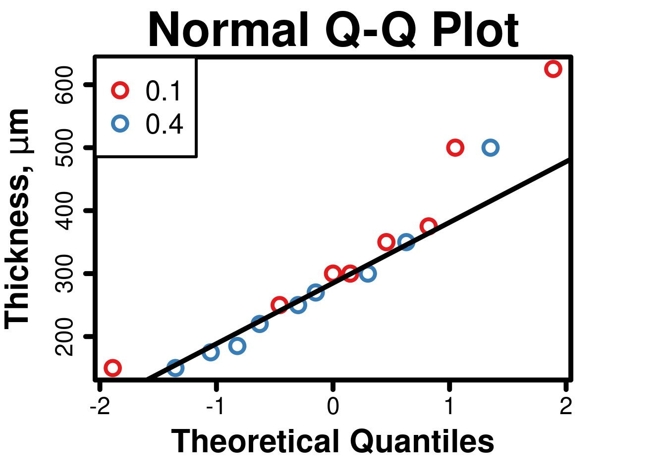
Atheroma thickness

Atheroma thickness data from Smith BW J Food Res 2013 (doi: 10.5539/jfr.v2n1p168).

Import dataset

jfr2013_atheroma <- read.table('data/t_test_jfr2013_atheroma.csv',
                               header = TRUE,
                               sep = ',')
attach(jfr2013_atheroma)
names(jfr2013_atheroma)

## [1] "diet"      "thickness"

Perform t-test

The default assumes unequal variance and applies the Satterthwaite/Welch df modification.
var.equal = TRUE is used to specify equal variances and a pooled variance estimate.

t.test(
  jfr2013_atheroma$thickness ~ jfr2013_atheroma$diet,
  paired = FALSE,
  alternative = 'two.sided',
  var.equal = TRUE,
  conf.level = 0.95
)

## 
##  Two Sample t-test
## 
## data:  jfr2013_atheroma$thickness by jfr2013_atheroma$diet
## t = 1.4364, df = 15, p-value = 0.1714
## alternative hypothesis: true difference in means between group 0.1 and group 0.4 is not equal to 0
## 95 percent confidence interval:
##  -43.34361 222.51028
## sample estimates:
## mean in group 0.1 mean in group 0.4 
##          356.2500          266.6667

Test assumptions

The t test uses raw data, not residuals, so assumptions are tested using raw data.

Normality

The RColorBrewer package is loaded for additional colors, and a palette is added to R. Use brackets after vector name for specific colors when creating plots (for example: col=set1[4:14]).
Legend can also be manually positioned with xy coordinates (numbers from 0,0 at bottom left of whole plot to 1,1 at top right)

# Shapiro-Wilk W test
shapiro.test(thickness)

## 
##  Shapiro-Wilk normality test
## 
## data:  thickness
## W = 0.91231, p-value = 0.1094

# Normal Quantile-Quantile Plot
# Set graphical parameters
par(
  cex = 1,
  cex.main = 3,
  cex.lab = 2,
  font.lab = 2,
  cex.axis = 1.5,
  lwd = 5,
  lend = 0,
  ljoin = 0,
  tcl = -0.5,
  pch = 1,
  mar = c(5, 5, 3, 5)
)

# Load RColorBrewer and set palette
library(RColorBrewer)
set1 <- brewer.pal(8, 'Set1')

# Create vector for categories
categories <- factor(jfr2013_atheroma$diet)

# Create plot
qqnorm(
  jfr2013_atheroma$thickness,
  ylab = expression(bold(paste(
    'Thickness, ', mu, 'm'
  ))),
  axes = FALSE,
  col = set1[categories],
  lwd = 4,
  cex = 2
)
# Add normal line
qqline(jfr2013_atheroma$thickness, lwd = 5)
# Add border to complete axes
box(which = 'plot', bty = 'o', lwd = 5)
axis(1, lwd = 5, tcl = -0.5) # x axis
axis(2, lwd = 5, tcl = -0.5) # y axis
# Add legend
legend(
  'topleft',
  legend = levels(categories),
  box.lwd = 3,
  pch = 1.5,
  cex = 1.75,
  pt.cex = 2,
  pt.lwd = 4,
  col = set1
)

Equality of variances

var.test(jfr2013_atheroma$thickness ~ jfr2013_atheroma$diet)

## 
##  F test to compare two variances
## 
## data:  jfr2013_atheroma$thickness by jfr2013_atheroma$diet
## F = 1.8725, num df = 7, denom df = 8, p-value = 0.3983
## alternative hypothesis: true ratio of variances is not equal to 1
## 95 percent confidence interval:
##  0.4134808 9.1738855
## sample estimates:
## ratio of variances 
##           1.872473

Boxplot

Parameters (par): Graphical parameters need to be set again because of code chunk separation in RMarkdown. Normally they would only be set once per R session.
X axis: The default axes will usually detect categorical data and label axes accordingly, but categories will need to be specified for axes created separately. It is easiest to create a separate vector with the categories, and then reference it when creating the plot. Labels can also be specified with labels=c('group1', 'group2').
Y axis: Note that it does not always start at zero, but encompasses the data range with some padding.

# Set graphical parameters
par(
  cex = 1,
  cex.main = 3,
  cex.lab = 2,
  font.lab = 2,
  cex.axis = 1.5,
  lwd = 5,
  lend = 0,
  ljoin = 0,
  tcl = -0.5,
  pch = 1,
  mar = c(5, 5, 3, 5)
)

# Create boxplot
boxplot(
  jfr2013_atheroma$thickness ~ jfr2013_atheroma$diet,
  main = 'Atheroma Thickness',
  xlab = 'Diet',
  ylab = expression(bold(paste(
    'Thickness, ', mu, 'm'
  ))),
  axes = FALSE,
  lwd = 4,
  medlwd = 7,
  outlwd = 4,
  cex = 2,
  col = set1
)

# Add border to complete axes
box(which = 'plot', bty = 'l', lwd = 5)

# Create vector with means of each group
means <- aggregate(thickness ~ diet, jfr2013_atheroma, mean)
# Add points for group means to boxplot
points(
  means$thickness,
  cex = 2,
  pch = 23,
  bg = 0,
  lwd = 4
)

# X axis
axis(
  1,
  lwd = 5,
  tcl = -0.5,
  labels = levels(categories),
  at = c(1:2)
)

# Y axis
axis(2, lwd = 5, tcl = -0.5)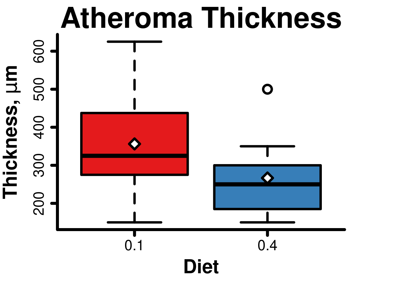

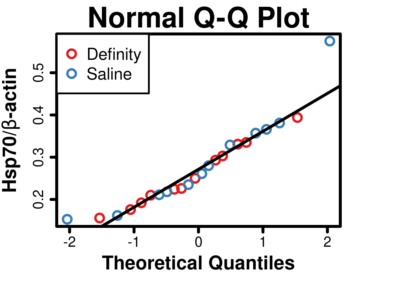
Aorta Hsp70

Aorta Hsp70 data from Smith BW J Ultrasound Med 2015 (doi: 10.7863/ultra.34.7.1209).

Import dataset

AortaHsp70 <- read.table('data/t_test_jum2015_hsp70.csv',
                         header = TRUE,
                         sep = ',')
attach(AortaHsp70)
names(AortaHsp70)

## [1] "exposure" "Hsp70"

Perform t-test

The default assumes unequal variance and applies the Satterthwaite/Welch df modification.
var.equal = TRUE is used to specify equal variances and a pooled variance estimate.

t.test(
  AortaHsp70$Hsp70 ~ AortaHsp70$exposure,
  paired = FALSE,
  alternative = 'two.sided',
  var.equal = TRUE,
  conf.level = 0.95
)

## 
##  Two Sample t-test
## 
## data:  AortaHsp70$Hsp70 by AortaHsp70$exposure
## t = -0.91363, df = 22, p-value = 0.3708
## alternative hypothesis: true difference in means between group Definity and group Saline is not equal to 0
## 95 percent confidence interval:
##  -0.11935215  0.04635215
## sample estimates:
## mean in group Definity   mean in group Saline 
##                 0.2575                 0.2940

Test assumptions

The t test uses raw data, not residuals, so assumptions are tested using raw data.

Normality

The RColorBrewer package is loaded for additional colors, and a palette is added to R. Use brackets after vector name for specific colors when creating plots (for example: col=set1[4:14]).
Legend can also be manually positioned with xy coordinates (numbers from 0,0 at bottom left of whole plot to 1,1 at top right)

# Shapiro-Wilk W test
shapiro.test(AortaHsp70$Hsp70)

## 
##  Shapiro-Wilk normality test
## 
## data:  AortaHsp70$Hsp70
## W = 0.90895, p-value = 0.03347

# Normal Quantile-Quantile Plot
# Set graphical parameters
par(
  cex = 1,
  cex.main = 3,
  cex.lab = 2,
  font.lab = 2,
  cex.axis = 1.5,
  lwd = 5,
  lend = 0,
  ljoin = 0,
  tcl = -0.5,
  pch = 1,
  mar = c(5, 5, 3, 5)
)

# Load RColorBrewer and set palette
library(RColorBrewer)
set1 <- brewer.pal(8, 'Set1')

# Create vector for categories
categories <- factor(AortaHsp70$exposure)

# Create plot
qqnorm(
  Hsp70,
  ylab = expression(bold(paste(
    'Hsp70/', beta, '-actin'
  ))),
  axes = FALSE,
  col = set1[categories],
  lwd = 4,
  cex = 2
)
# Add normal line
qqline(AortaHsp70$Hsp70, lwd = 5)
# Add border to complete axes
box(which = 'plot', bty = 'o', lwd = 5)
axis(1, lwd = 5, tcl = -0.5) # x axis
axis(2, lwd = 5, tcl = -0.5) # y axis
# Add legend
legend(
  'topleft',
  legend = levels(categories),
  box.lwd = 3,
  pch = 1.5,
  cex = 1.75,
  pt.cex = 2,
  pt.lwd = 4,
  col = set1
)

Equality of variances

var.test(AortaHsp70$Hsp70 ~ AortaHsp70$exposure)

## 
##  F test to compare two variances
## 
## data:  AortaHsp70$Hsp70 by AortaHsp70$exposure
## F = 0.38929, num df = 11, denom df = 11, p-value = 0.1328
## alternative hypothesis: true ratio of variances is not equal to 1
## 95 percent confidence interval:
##  0.1120669 1.3522650
## sample estimates:
## ratio of variances 
##          0.3892868

Boxplot

Parameters (par): Graphical parameters need to be set again because of code chunk separation in RMarkdown. Normally they would only be set once per R session.
X axis: The default axes will usually detect categorical data and label axes accordingly, but categories will need to be specified for axes created separately. It is easiest to create a separate vector with the categories, and then reference it when creating the plot. Labels can also be specified with labels=c('group1', 'group2').
Y axis: Note that it does not always start at zero, but encompasses the data range with some padding.

# Set graphical parameters
par(
  cex = 1,
  cex.main = 3,
  cex.lab = 2,
  font.lab = 2,
  cex.axis = 1.5,
  lwd = 5,
  lend = 0,
  ljoin = 0,
  tcl = -0.5,
  pch = 1,
  mar = c(5, 5, 3, 5)
)

# Create boxplot
boxplot(
  AortaHsp70$Hsp70 ~ AortaHsp70$exposure,
  main = 'Aorta Hsp70',
  xlab = 'Exposure',
  ylab = expression(bold(paste(
    'Hsp70/', beta, '-actin'
  ))),
  axes = FALSE,
  lwd = 4,
  medlwd = 7,
  outlwd = 4,
  cex = 2,
  col = set1
)

# Add border to complete axes
box(which = 'plot', bty = 'l', lwd = 5)

# Create vector with means of each group
means <- aggregate(Hsp70 ~ exposure, AortaHsp70, mean)
# Add points for group means to boxplot
points(
  means$Hsp70,
  cex = 2,
  pch = 23,
  bg = 0,
  lwd = 4
)

# X axis
axis(
  1,
  lwd = 5,
  tcl = -0.5,
  labels = levels(categories),
  at = c(1:2)
)

# Y axis
axis(2, lwd = 5, tcl = -0.5)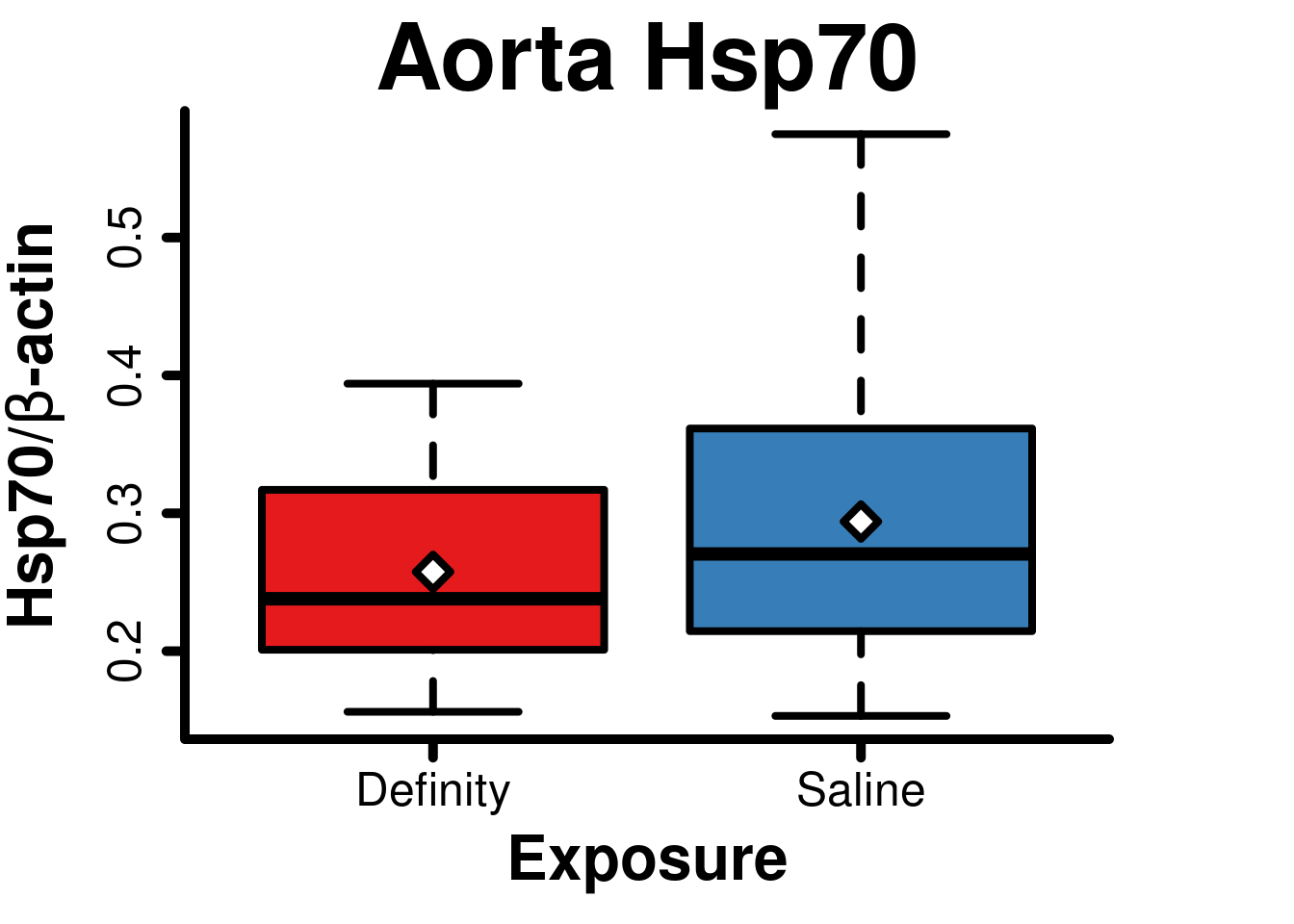

Linear regression

Simple linear regression aztcpm

aztcpm dataset from University of Illinois statistics course PATH 591 lab 02 and PATH 591 lecture 04 A

Intro

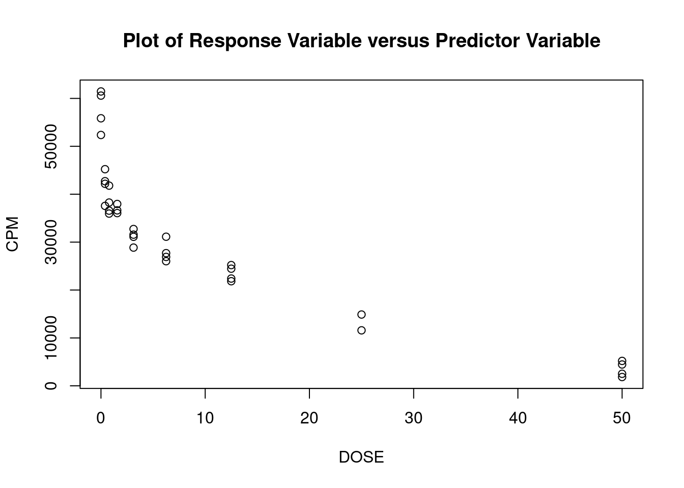
These data are from an in-vitro study of the effect of AZT dose on DNA replication (CPM) for FeLV (feline leukemia virus). (The experimental unit is the cell culture sample). For the linear regression analysis, the dependent variable is CPM (counts per minute, indicating quantity of Feline Leukemia Virus DNA in a cell culture) and the independent (predictor) variable is DOSE (dose of AZT).

Import dataset

aztcpm <- read.table('data/lm_aztcpm.csv', header = TRUE, sep = ',')
attach(aztcpm)
names(aztcpm)

## [1] "DOSE" "CPM"

Perform linear regression

lm1 <- lm(CPM ~ DOSE)

Perform regression diagnostics and test assumptions

library(gvlma)
gvlmalm1 <- gvlma(lm1)
summary(gvlmalm1)

## 
## Call:
## lm(formula = CPM ~ DOSE)
## 
## Residuals:
##    Min     1Q Median     3Q    Max 
##  -8712  -5708  -2483   3224  21640 
## 
## Coefficients:
##             Estimate Std. Error t value Pr(>|t|)    
## (Intercept) 39810.58    1711.46  23.261  < 2e-16 ***
## DOSE         -813.61      89.45  -9.096 2.93e-10 ***
## ---
## Signif. codes:  0 '***' 0.001 '**' 0.01 '*' 0.05 '.' 0.1 ' ' 1
## 
## Residual standard error: 8215 on 31 degrees of freedom
## Multiple R-squared:  0.7274, Adjusted R-squared:  0.7186 
## F-statistic: 82.73 on 1 and 31 DF,  p-value: 2.931e-10
## 
## 
## ASSESSMENT OF THE LINEAR MODEL ASSUMPTIONS
## USING THE GLOBAL TEST ON 4 DEGREES-OF-FREEDOM:
## Level of Significance =  0.05 
## 
## Call:
##  gvlma(x = lm1) 
## 
##                     Value   p-value                   Decision
## Global Stat        32.863 1.274e-06 Assumptions NOT satisfied!
## Skewness            9.168 2.463e-03 Assumptions NOT satisfied!
## Kurtosis            1.413 2.346e-01    Assumptions acceptable.
## Link Function      12.218 4.733e-04 Assumptions NOT satisfied!
## Heteroscedasticity 10.064 1.512e-03 Assumptions NOT satisfied!

shapiro.test(rstandard(lm1))

## 
##  Shapiro-Wilk normality test
## 
## data:  rstandard(lm1)
## W = 0.85782, p-value = 0.0005083

cor.test(fitted(lm1), abs(rstandard(lm1)), method = 'spearman')

## Warning in cor.test.default(fitted(lm1), abs(rstandard(lm1)), method =
## "spearman"): Cannot compute exact p-value with ties

## 
##  Spearman's rank correlation rho
## 
## data:  fitted(lm1) and abs(rstandard(lm1))
## S = 6143.9, p-value = 0.8827
## alternative hypothesis: true rho is not equal to 0
## sample estimates:
##         rho 
## -0.02671635

library(car)

## Loading required package: carData

durbinWatsonTest(lm1)

##  lag Autocorrelation D-W Statistic p-value
##    1        0.797716     0.1772224       0
##  Alternative hypothesis: rho != 0

outlierTest(lm1)

## No Studentized residuals with Bonferroni p < 0.05
## Largest |rstudent|:
##    rstudent unadjusted p-value Bonferroni p
## 33 3.027239          0.0050324      0.16607

Generate plots

plot(gvlmalm1, onepage = FALSE)

plot(lm1, which = 3:5)

acf(rstandard(lm1), main = 'Autocorrelation plot')

Log transform

lmlog <- update(lm1, log(CPM) ~ DOSE)

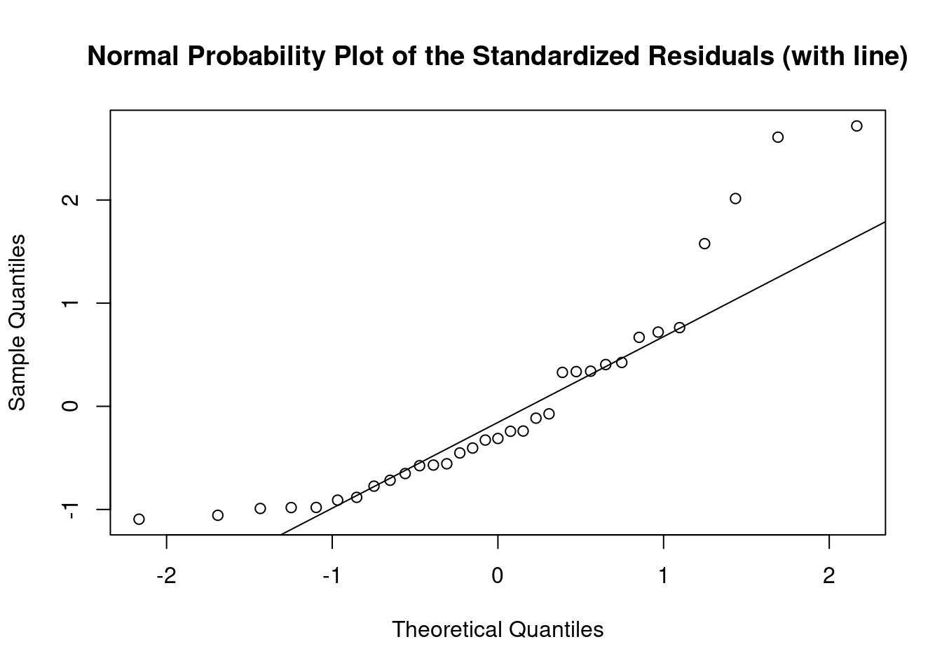
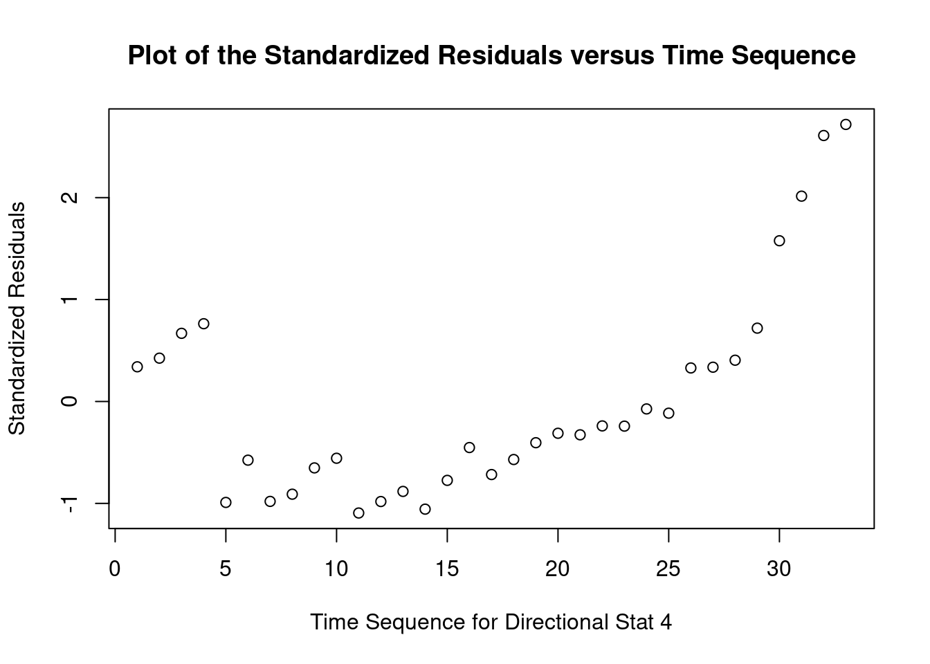
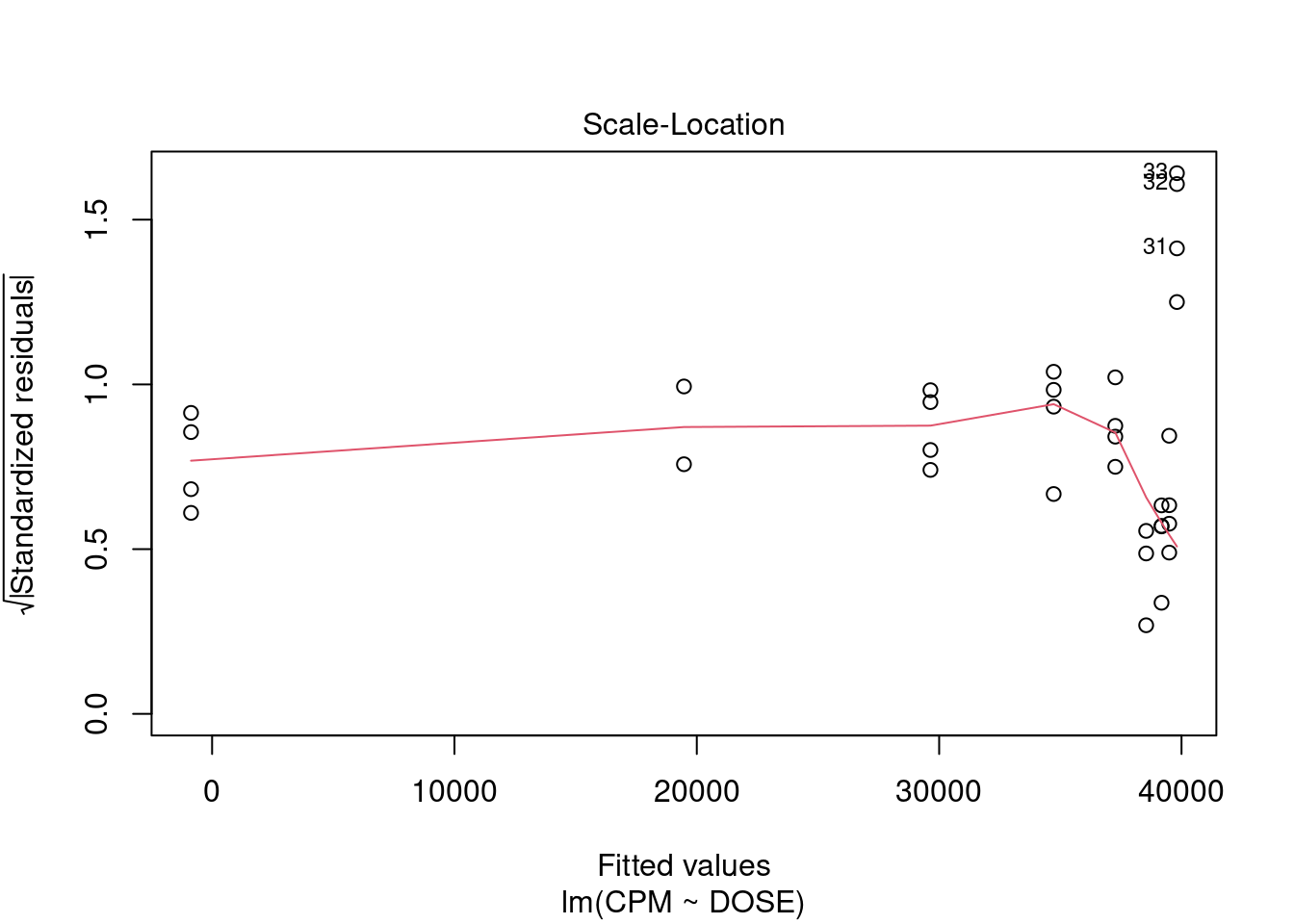
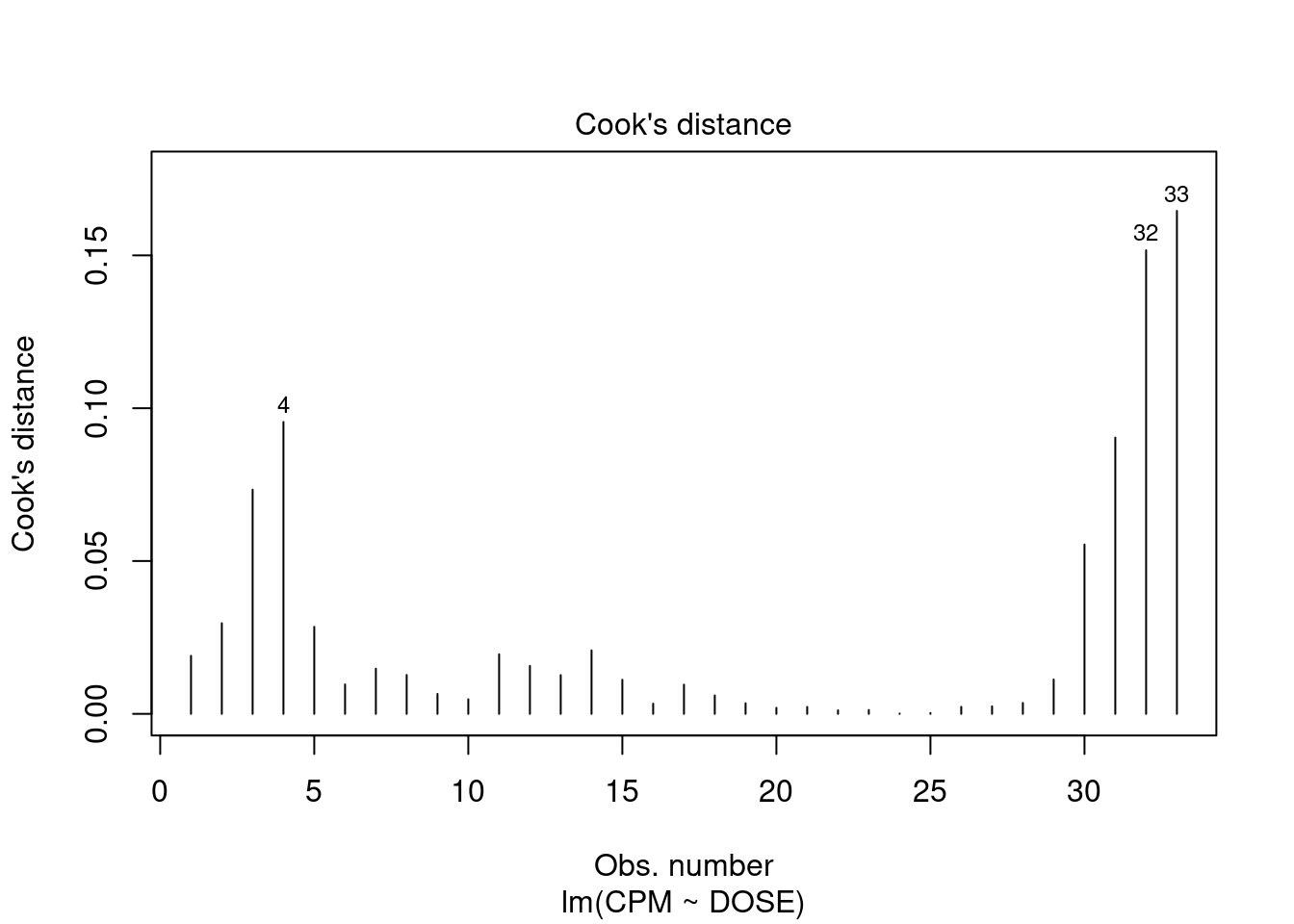
Perform regression diagnostics and test assumptions

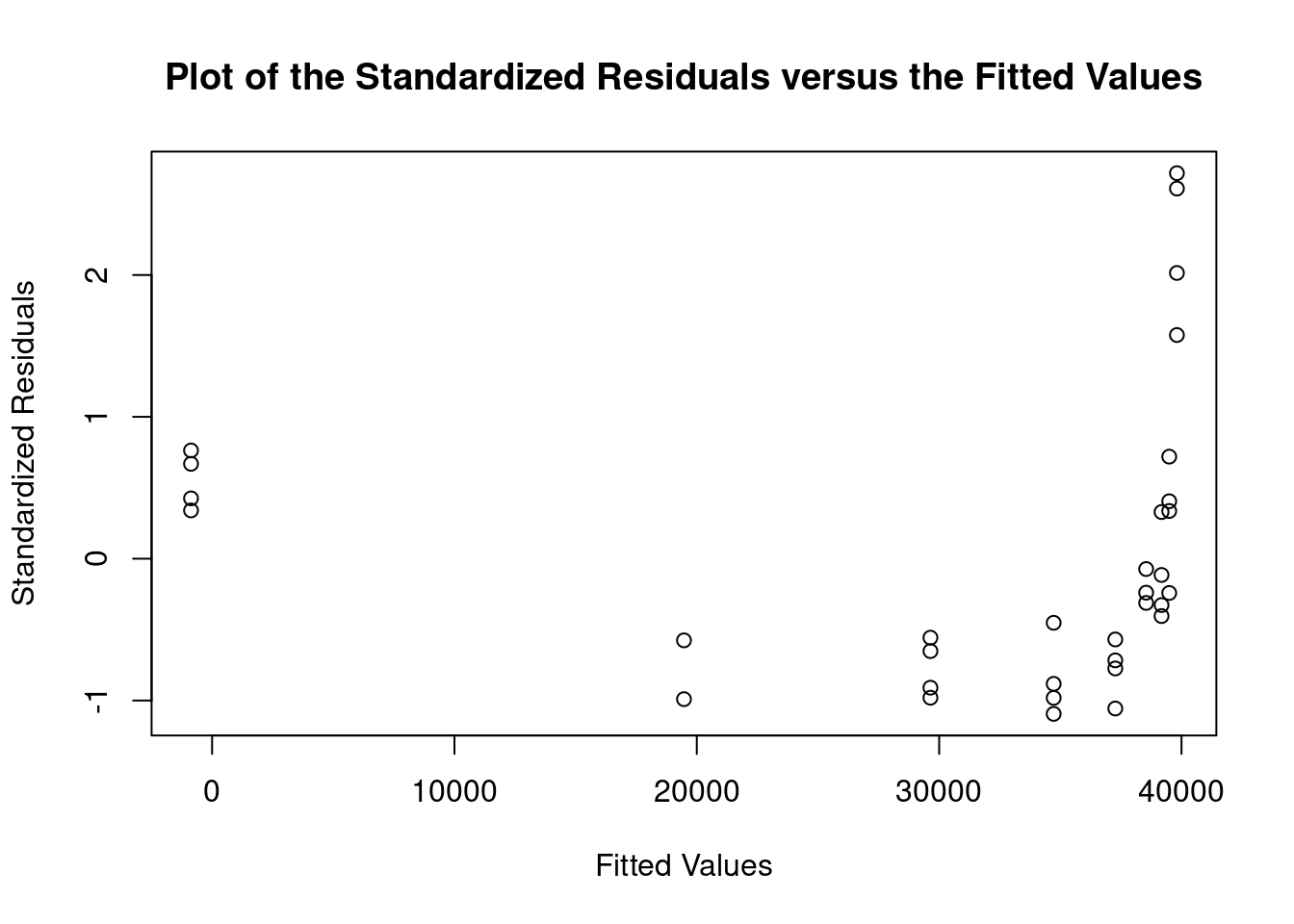
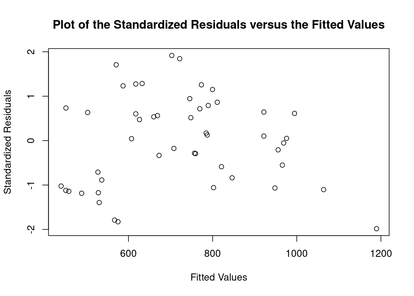
Log transformation improves compliance with linear model assumptions. Some serial correlation remains, which is evident in plots of residuals vs fitted values and in the significant result of the Durbin-Watson D test, but it is within acceptable limits of the global validation of linear model assumptions.

library(gvlma)
gvlmalog <- gvlma(lmlog)
summary(gvlmalog)

## 
## Call:
## lm(formula = log(CPM) ~ DOSE)
## 
## Residuals:
##      Min       1Q   Median       3Q      Max 
## -0.57193 -0.11370 -0.02660  0.08659  0.46827 
## 
## Coefficients:
##             Estimate Std. Error t value Pr(>|t|)    
## (Intercept) 10.66086    0.04420  241.20   <2e-16 ***
## DOSE        -0.05144    0.00231  -22.27   <2e-16 ***
## ---
## Signif. codes:  0 '***' 0.001 '**' 0.01 '*' 0.05 '.' 0.1 ' ' 1
## 
## Residual standard error: 0.2122 on 31 degrees of freedom
## Multiple R-squared:  0.9412, Adjusted R-squared:  0.9393 
## F-statistic: 495.8 on 1 and 31 DF,  p-value: < 2.2e-16
## 
## 
## ASSESSMENT OF THE LINEAR MODEL ASSUMPTIONS
## USING THE GLOBAL TEST ON 4 DEGREES-OF-FREEDOM:
## Level of Significance =  0.05 
## 
## Call:
##  gvlma(x = lmlog) 
## 
##                       Value p-value                Decision
## Global Stat        3.952318 0.41250 Assumptions acceptable.
## Skewness           0.056280 0.81248 Assumptions acceptable.
## Kurtosis           0.676082 0.41094 Assumptions acceptable.
## Link Function      0.004124 0.94880 Assumptions acceptable.
## Heteroscedasticity 3.215833 0.07293 Assumptions acceptable.

shapiro.test(rstandard(lmlog))

## 
##  Shapiro-Wilk normality test
## 
## data:  rstandard(lmlog)
## W = 0.94082, p-value = 0.07176

cor.test(fitted(lmlog), abs(rstandard(lmlog)), method = 'spearman')

## Warning in cor.test.default(fitted(lmlog), abs(rstandard(lmlog)), method =
## "spearman"): Cannot compute exact p-value with ties

## 
##  Spearman's rank correlation rho
## 
## data:  fitted(lmlog) and abs(rstandard(lmlog))
## S = 6684, p-value = 0.5168
## alternative hypothesis: true rho is not equal to 0
## sample estimates:
##        rho 
## -0.1169866

library(car)
durbinWatsonTest(lmlog)

##  lag Autocorrelation D-W Statistic p-value
##    1       0.4659162     0.7381887       0
##  Alternative hypothesis: rho != 0

outlierTest(lmlog)

##    rstudent unadjusted p-value Bonferroni p
## 1 -3.574629          0.0012106      0.03995

Generate plots

plot(gvlmalog, onepage = FALSE)

plot(lmlog, which = 3:5)

acf(rstandard(lmlog), main = 'Autocorrelation plot')

Simple linear regression jfs data

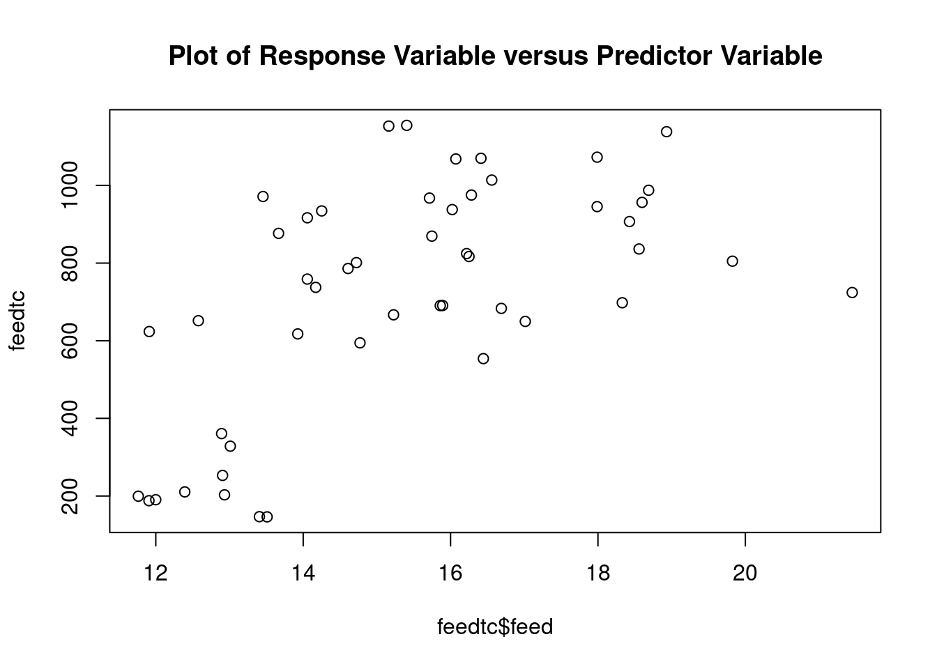
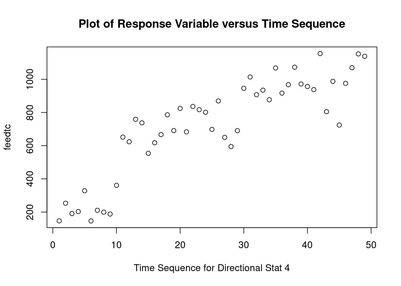
Feed intake vs total cholesterol data from Smith BW J Food Sci 2015 (doi: 10.1111/1750-3841.12968).

Import dataset

feedtc <- read.table('data/lm_jfs2015_feed_vs_tc.csv',
                     header = TRUE,
                     sep = ',')
attach(feedtc)
names(feedtc)

## [1] "id"   "diet" "tc"   "feed"

Perform linear regression

feedtclm1 <- lm(feedtc$tc ~ feedtc$feed)

Perform regression diagnostics and test assumptions

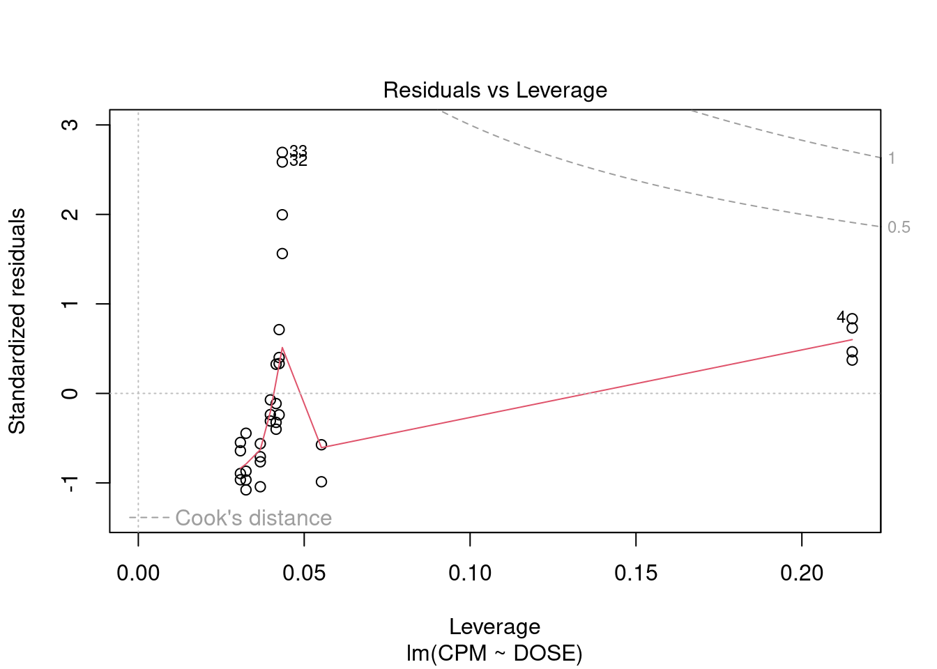
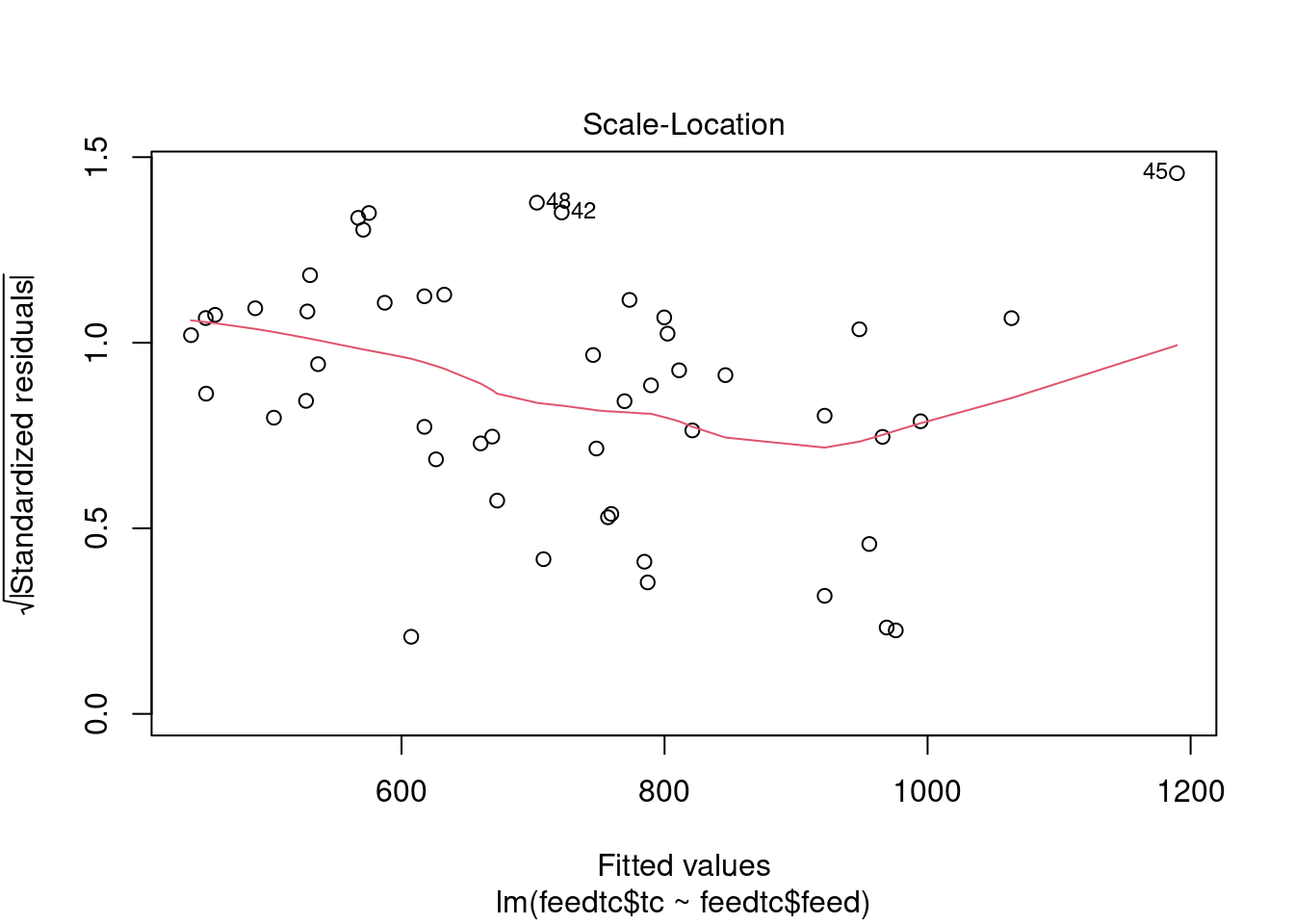
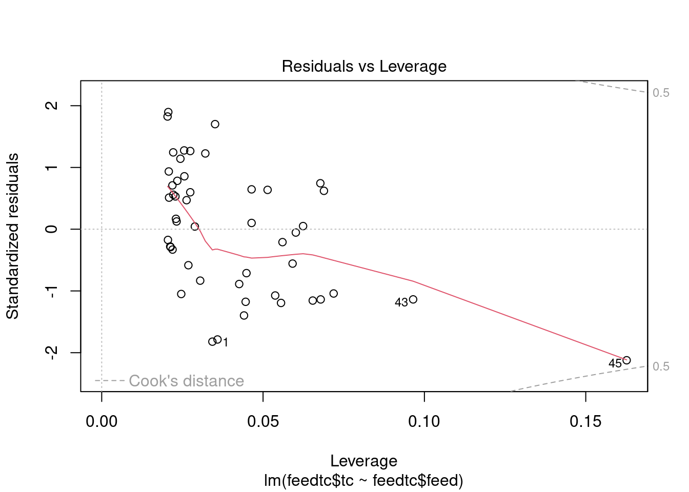
The dataset contains some potential outliers (M1356 and M1376), and a violation of the link function according to gvlma.

Outliers
- The major outlier is M1376, which returns a Cook’s D value of 0.43. This may or may not be an outlier, depending on the definition. It is just under the critical F value (F0.50(1,40)=0.463).
- The Bonferroni outlier test does not identify any outliers either.
- However, according to R in Action 8.4.3, Cook’s D values greater than 4/(n-k-1), where n is the sample size and k is the number of predictor variables, indicate influential observations (though he usually uses a cutoff of 1). M1376 would be considered an outlier by this definition.
Link function
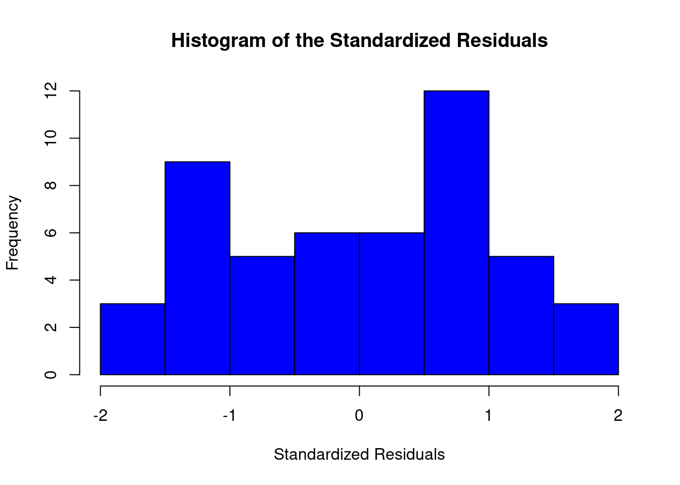
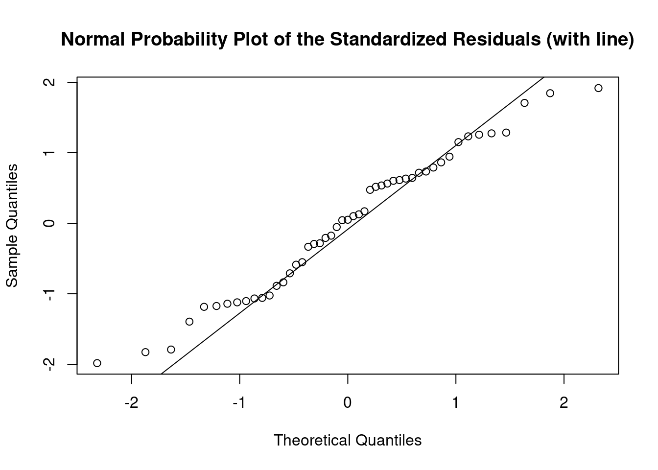
- The link function violation is difficult to address. The dataset conforms to a normal distribution as evidenced by the normal probability plot and Shapiro-Wilk W test, so it would not seem like a concern, but it is enough to violate gvlma. However, this doesn’t seem like a situation where it would be neccessary to switch to another model (such as a generalized linear mixed model) and specify a different link function.
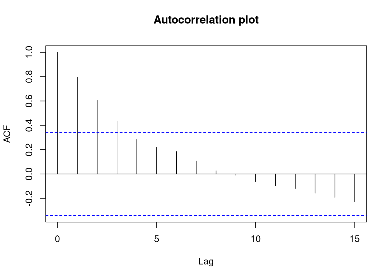
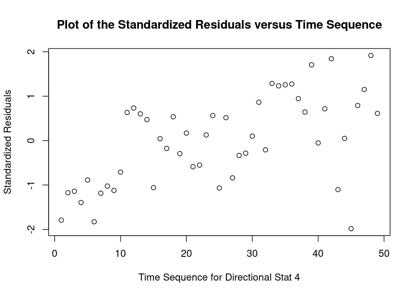
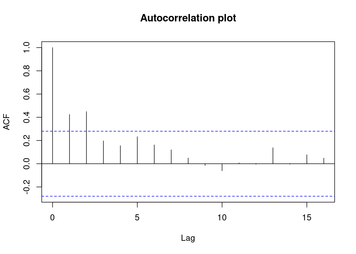
- The Spearman rank order correlation between absolute values of residuals and predicted values returns a significant result, but heteroscedasticity is within acceptable limits according to gvlma and by visual inspection of plots of residuals vs. fitted values and autocorrelation.

library(gvlma)
feedtcgvlmalm1 <- gvlma(feedtclm1)
summary(feedtcgvlmalm1)

## 
## Call:
## lm(formula = feedtc$tc ~ feedtc$feed)
## 
## Residuals:
##     Min      1Q  Median      3Q     Max 
## -465.42 -208.18   11.74  168.20  449.91 
## 
## Coefficients:
##             Estimate Std. Error t value Pr(>|t|)    
## (Intercept)  -470.33     232.65  -2.022   0.0489 *  
## feedtc$feed    77.39      14.94   5.179 4.58e-06 ***
## ---
## Signif. codes:  0 '***' 0.001 '**' 0.01 '*' 0.05 '.' 0.1 ' ' 1
## 
## Residual standard error: 239.6 on 47 degrees of freedom
## Multiple R-squared:  0.3633, Adjusted R-squared:  0.3498 
## F-statistic: 26.82 on 1 and 47 DF,  p-value: 4.578e-06
## 
## 
## ASSESSMENT OF THE LINEAR MODEL ASSUMPTIONS
## USING THE GLOBAL TEST ON 4 DEGREES-OF-FREEDOM:
## Level of Significance =  0.05 
## 
## Call:
##  gvlma(x = feedtclm1) 
## 
##                       Value   p-value                   Decision
## Global Stat        15.17502 0.0043516 Assumptions NOT satisfied!
## Skewness            0.03692 0.8476301    Assumptions acceptable.
## Kurtosis            1.62599 0.2022584    Assumptions acceptable.
## Link Function      13.31102 0.0002639 Assumptions NOT satisfied!
## Heteroscedasticity  0.20109 0.6538402    Assumptions acceptable.

shapiro.test(rstandard(feedtclm1))

## 
##  Shapiro-Wilk normality test
## 
## data:  rstandard(feedtclm1)
## W = 0.97342, p-value = 0.3295

cor.test(fitted(feedtclm1), abs(rstandard(feedtclm1)), method = 'spearman')

## Warning in cor.test.default(fitted(feedtclm1), abs(rstandard(feedtclm1)), :
## Cannot compute exact p-value with ties

## 
##  Spearman's rank correlation rho
## 
## data:  fitted(feedtclm1) and abs(rstandard(feedtclm1))
## S = 25966, p-value = 0.02278
## alternative hypothesis: true rho is not equal to 0
## sample estimates:
##        rho 
## -0.3248125

library(car)
durbinWatsonTest(feedtclm1)

##  lag Autocorrelation D-W Statistic p-value
##    1       0.4305706      1.065764       0
##  Alternative hypothesis: rho != 0

outlierTest(feedtclm1)

## No Studentized residuals with Bonferroni p < 0.05
## Largest |rstudent|:
##     rstudent unadjusted p-value Bonferroni p
## 45 -2.208409           0.032238           NA

Generate plots

plot(feedtcgvlmalm1, onepage = FALSE)

plot(feedtclm1, which = 3)

cookscritical <- 4 / (nrow(feedtc) - length(feedtclm1$coefficients) - 2)
plot(feedtclm1, which = 4, cook.levels = cookscritical)
abline(h = cookscritical, lty = 2, col = 'red')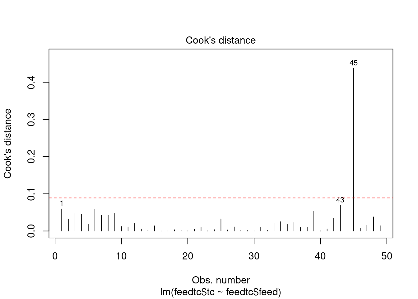

plot(feedtclm1, which = 5)

acf(rstandard(feedtclm1), main = 'Autocorrelation plot')

Calculate Spearman correlation

The Spearman rank order correlation between the independent and dependent variable is another type of correlation that is more widely valid, especially in situations where F test assumptions are violated.

cor.test(feedtc$tc, feedtc$feed, method = 'spearman')

## Warning in cor.test.default(feedtc$tc, feedtc$feed, method = "spearman"):
## Cannot compute exact p-value with ties

## 
##  Spearman's rank correlation rho
## 
## data:  feedtc$tc and feedtc$feed
## S = 8028.4, p-value = 8.003e-06
## alternative hypothesis: true rho is not equal to 0
## sample estimates:
##       rho 
## 0.5903873

Multiple linear regression and ANOVA example

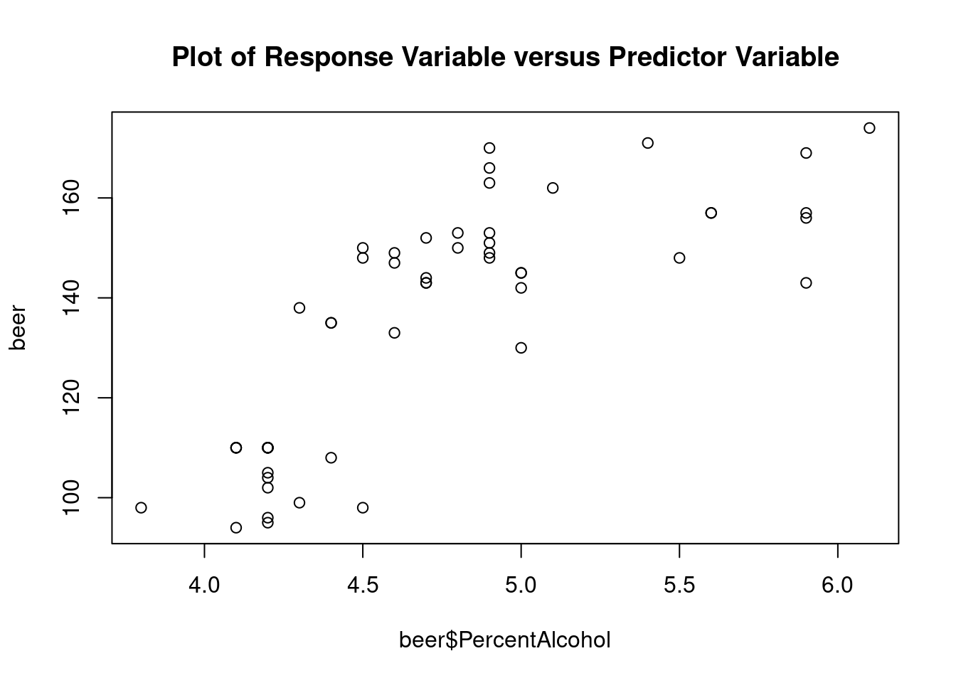
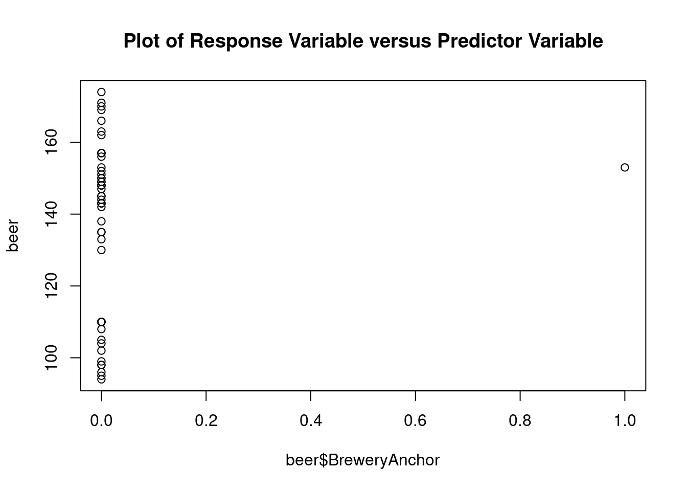
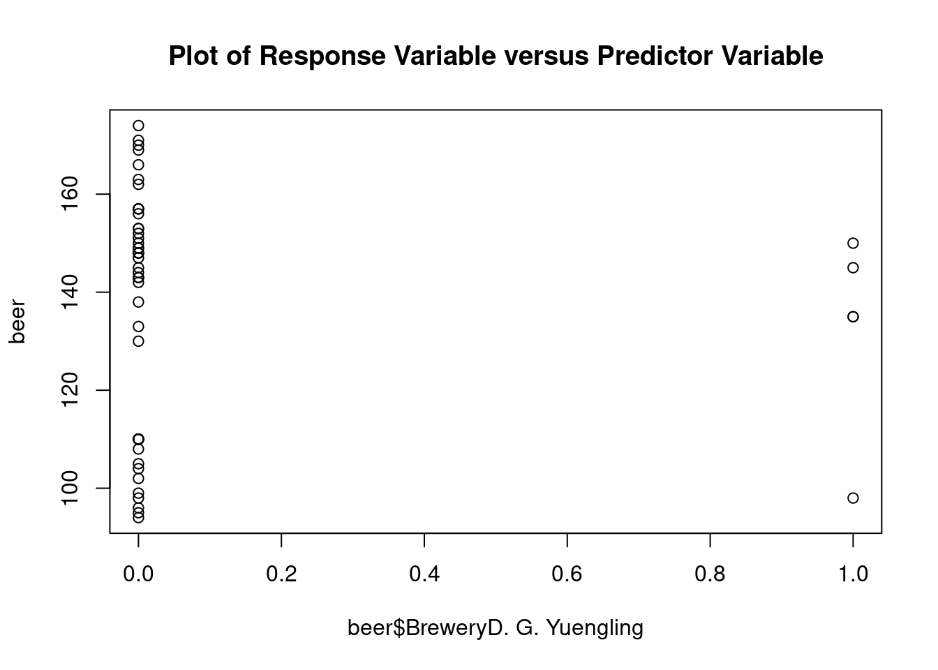
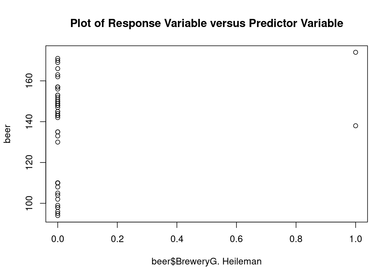
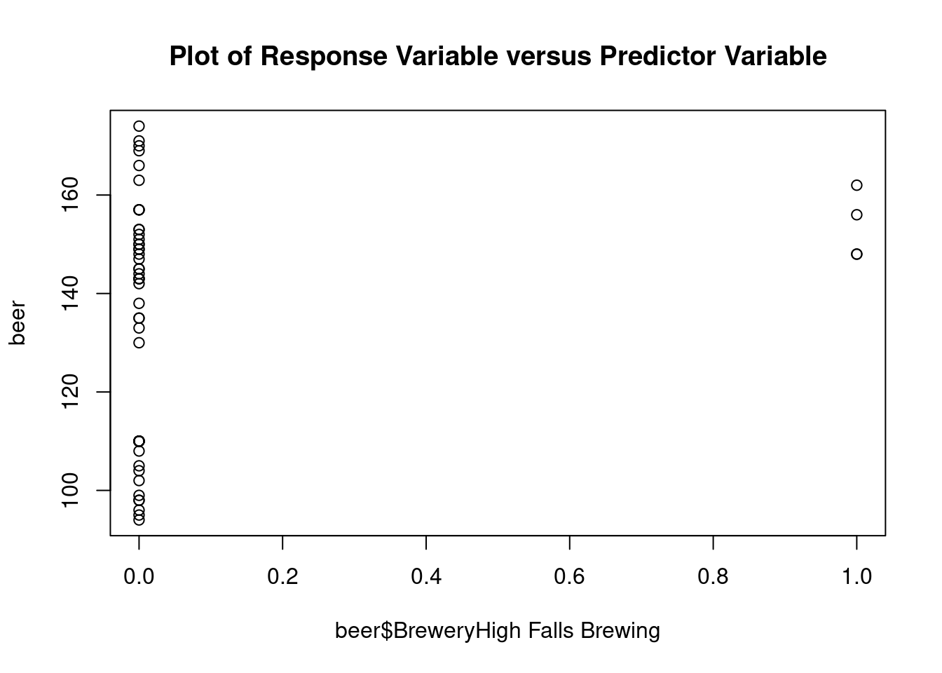
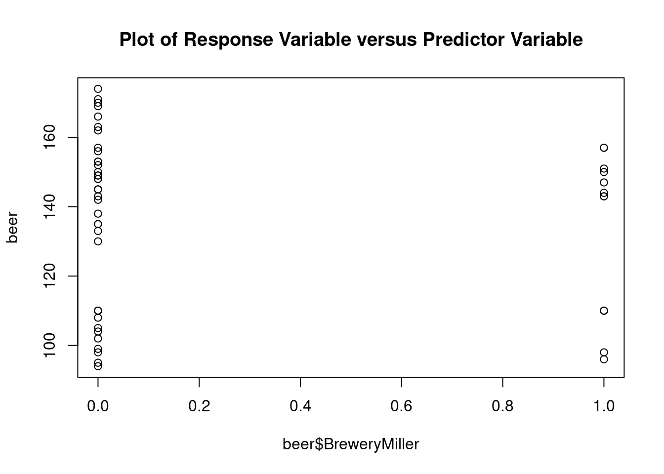
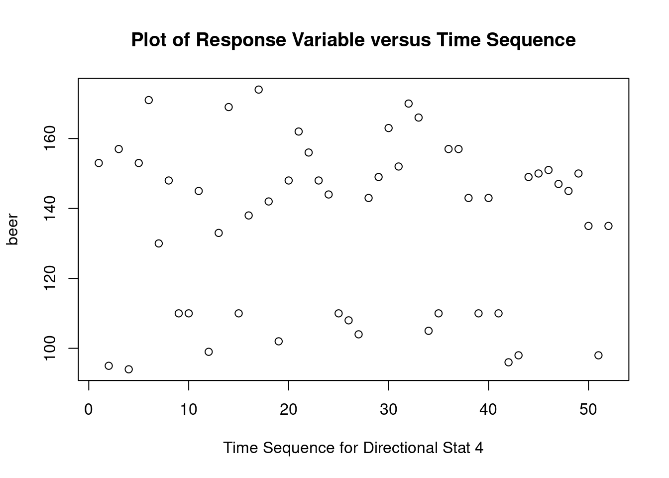
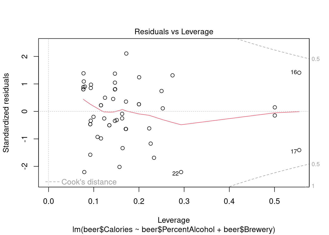
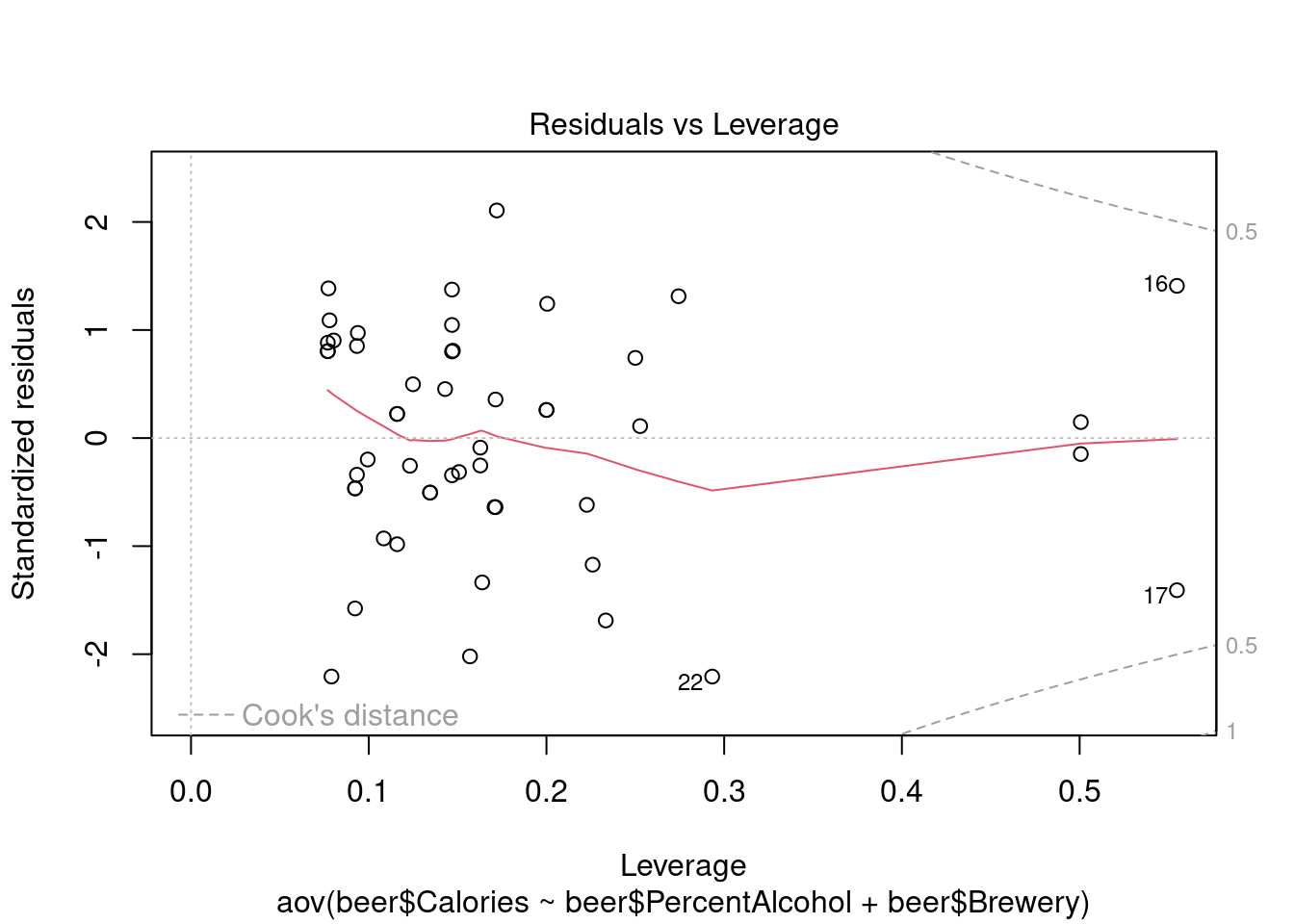
This dataset from Doug Simpson at University of Illinois contains information on the number of calories in various beers, along with their percent alcohol and brewery.

PercentAlcohol is a quantitative continuous independent variable and Brewery is a categorical independent variable.

Import dataset

beer <- read.table('data/anova_mlr_beer.csv', header = TRUE, sep = ',')
attach(beer)

Perform multiple linear regression in lm

beerlm1 <- lm(beer$Calories ~ beer$PercentAlcohol + beer$Brewery)
anova(beerlm1)

## Analysis of Variance Table
## 
## Response: beer$Calories
##                     Df  Sum Sq Mean Sq  F value  Pr(>F)    
## beer$PercentAlcohol  1 17914.2 17914.2 102.3698 7.9e-13 ***
## beer$Brewery         8  4424.9   553.1   3.1608 0.00682 ** 
## Residuals           42  7349.8   175.0                     
## ---
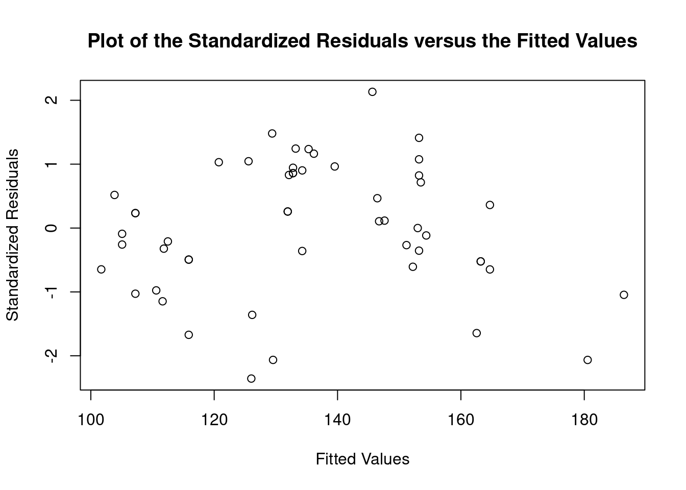
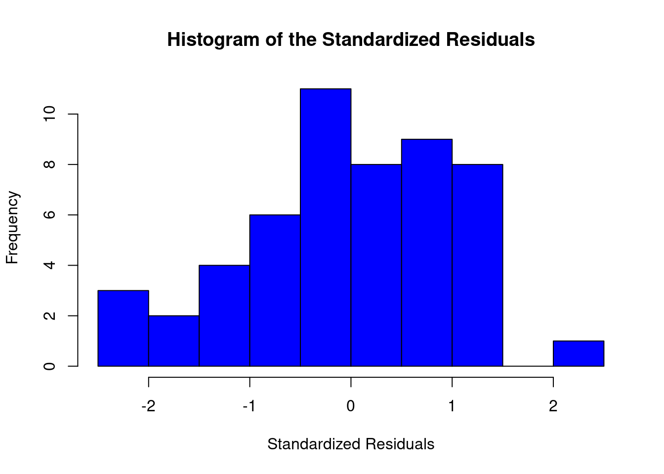
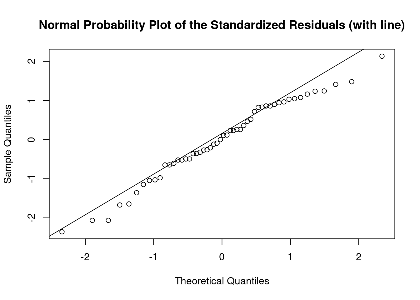
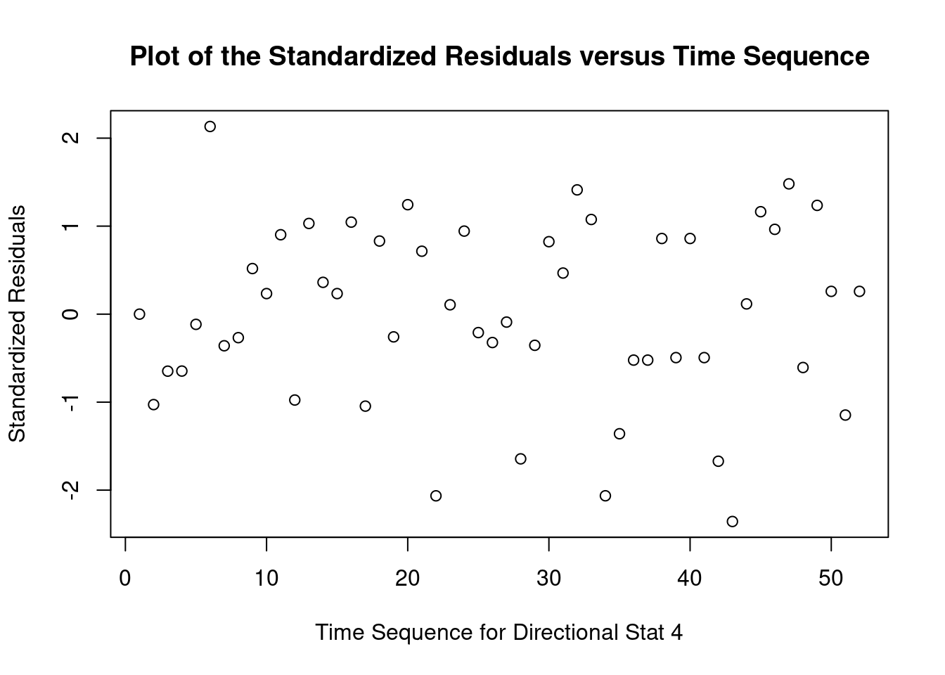
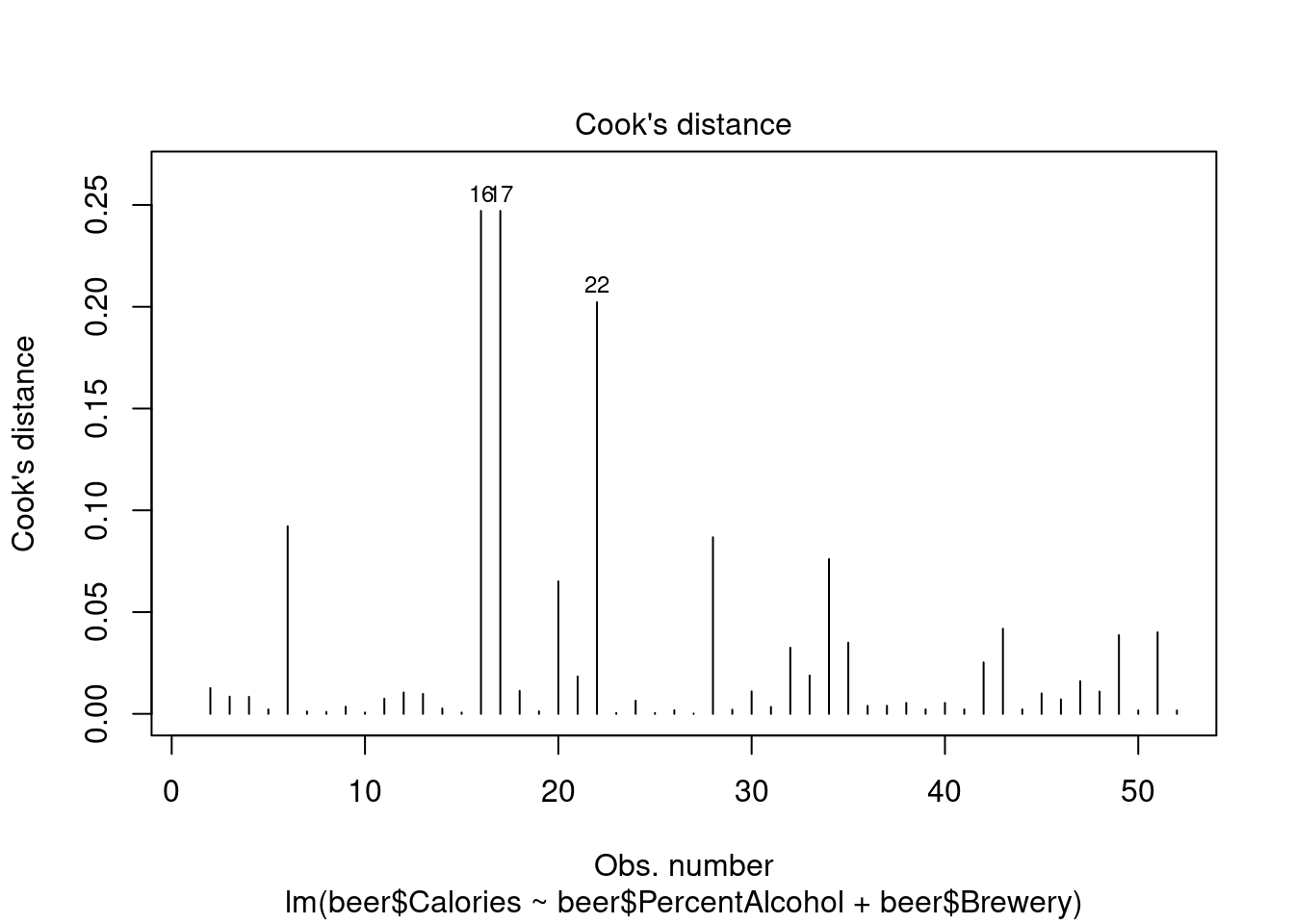
## Signif. codes:  0 '***' 0.001 '**' 0.01 '*' 0.05 '.' 0.1 ' ' 1

Perform regression diagnostics and test assumptions

library(gvlma)
beergvlmalm1 <- gvlma(beerlm1)
summary(beergvlmalm1)

## 
## Call:
## lm(formula = beer$Calories ~ beer$PercentAlcohol + beer$Brewery)
## 
## Residuals:
##      Min       1Q   Median       3Q      Max 
## -28.0179  -6.4610   0.6312  10.2197  25.3521 
## 
## Coefficients:
##                                Estimate Std. Error t value Pr(>|t|)    
## (Intercept)                     -36.937     17.061  -2.165  0.03612 *  
## beer$PercentAlcohol              33.812      3.439   9.831 1.86e-12 ***
## beer$BreweryAnchor               24.258     14.152   1.714  0.09389 .  
## beer$BreweryAnheuser Busch        2.150      6.400   0.336  0.73858    
## beer$BreweryD. G. Yuengling      20.088      7.825   2.567  0.01391 *  
## beer$BreweryG. Heileman          17.115     10.722   1.596  0.11795    
## beer$BreweryHigh Falls Brewing   17.996      8.382   2.147  0.03762 *  
## beer$BreweryLeinenkugel          24.470      7.077   3.458  0.00126 ** 
## beer$BreweryMiller               10.801      6.206   1.740  0.08911 .  
## beer$BreweryPabst                29.021     10.607   2.736  0.00908 ** 
## ---
## Signif. codes:  0 '***' 0.001 '**' 0.01 '*' 0.05 '.' 0.1 ' ' 1
## 
## Residual standard error: 13.23 on 42 degrees of freedom
## Multiple R-squared:  0.7524, Adjusted R-squared:  0.6994 
## F-statistic: 14.18 on 9 and 42 DF,  p-value: 3.745e-10
## 
## 
## ASSESSMENT OF THE LINEAR MODEL ASSUMPTIONS
## USING THE GLOBAL TEST ON 4 DEGREES-OF-FREEDOM:
## Level of Significance =  0.05 
## 
## Call:
##  gvlma(x = beerlm1) 
## 
##                      Value   p-value                   Decision
## Global Stat        16.8557 0.0020618 Assumptions NOT satisfied!
## Skewness            1.0664 0.3017523    Assumptions acceptable.
## Kurtosis            0.3225 0.5700957    Assumptions acceptable.
## Link Function      14.4847 0.0001413 Assumptions NOT satisfied!
## Heteroscedasticity  0.9820 0.3216947    Assumptions acceptable.

shapiro.test(rstandard(beerlm1))

## 
##  Shapiro-Wilk normality test
## 
## data:  rstandard(beerlm1)
## W = 0.97308, p-value = 0.2957

cor.test(fitted(beerlm1), abs(rstandard(beerlm1)), method = 'spearman')

## Warning in cor.test.default(fitted(beerlm1), abs(rstandard(beerlm1)), method =
## "spearman"): Cannot compute exact p-value with ties

## 
##  Spearman's rank correlation rho
## 
## data:  fitted(beerlm1) and abs(rstandard(beerlm1))
## S = 19184, p-value = 0.3561
## alternative hypothesis: true rho is not equal to 0
## sample estimates:
##       rho 
## 0.1319358

library(car)
durbinWatsonTest(beerlm1)

##  lag Autocorrelation D-W Statistic p-value
##    1      0.07781896      1.843075   0.186
##  Alternative hypothesis: rho != 0

leveneTest(beer$Calories, beer$Brewery)

## Warning in leveneTest.default(beer$Calories, beer$Brewery): beer$Brewery
## coerced to factor.

## Levene's Test for Homogeneity of Variance (center = median)
##       Df F value Pr(>F)
## group  8  0.8577 0.5587
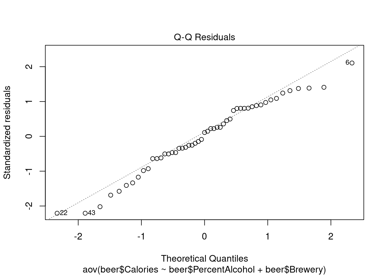
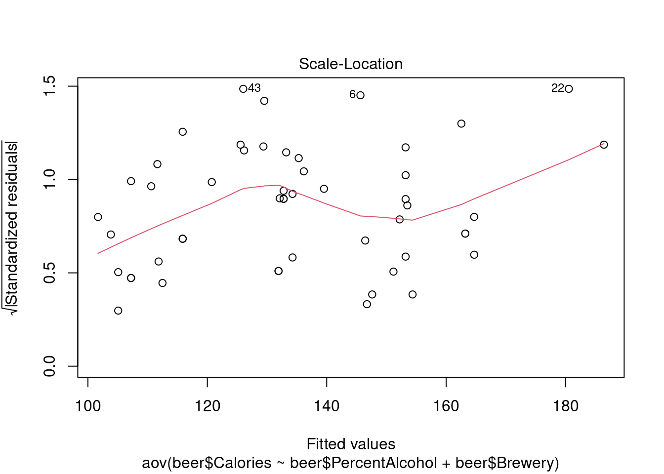
##       43

Generate plots

plot(beergvlmalm1, onepage = FALSE)

plot(beerlm1, which = 3:5)

## Warning: not plotting observations with leverage one:
##   1

Perform ANOVA in aov for comparison

beeraov1 <- aov(beer$Calories ~ beer$PercentAlcohol + beer$Brewery)
summary(beeraov1)

##                     Df Sum Sq Mean Sq F value  Pr(>F)    
## beer$PercentAlcohol  1  17914   17914 102.370 7.9e-13 ***
## beer$Brewery         8   4425     553   3.161 0.00682 ** 
## Residuals           42   7350     175                    
## ---
## Signif. codes:  0 '***' 0.001 '**' 0.01 '*' 0.05 '.' 0.1 ' ' 1

plot(beeraov1)

## Warning: not plotting observations with leverage one:
##   1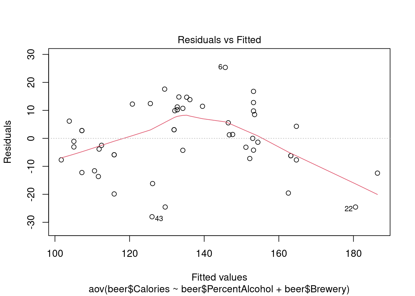

ANOVA

One-way ANOVA example

Gonadal adipose weights from Smith BW J Food Sci 2015 (doi: 10.1111/1750-3841.12968).

Import dataset

adipose_weights <-
  read.table('data/anova_one_way_jfs2015_adipose.csv',
             header = TRUE,
             sep = ',')
attach(adipose_weights)
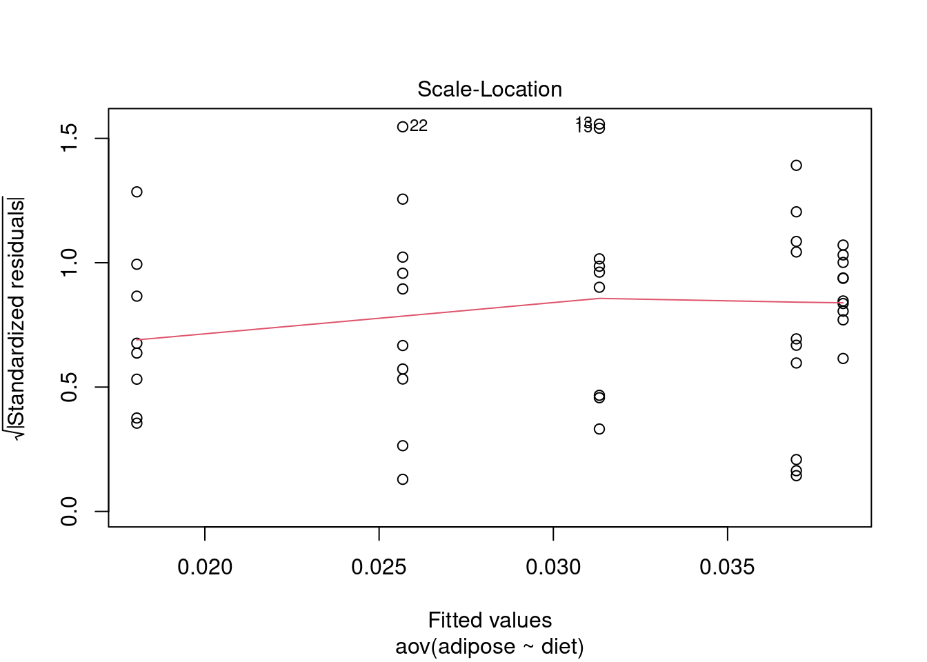
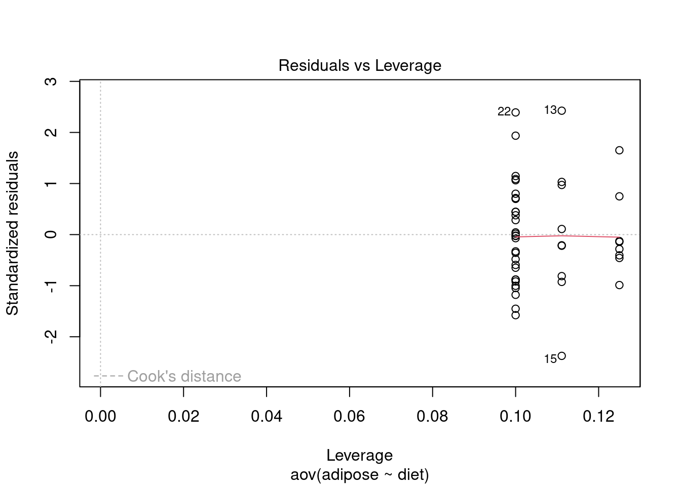
names(adipose_weights)

## [1] "id"      "diet"    "adipose"

Perform ANOVA in aov

# Convert independent variable to a factor for use later by glht()
adipose_weights$diet <- as.factor(adipose_weights$diet)
# Perform ANOVA
adiposeaov1 <- aov(adipose ~ diet, data = adipose_weights)
summary(adiposeaov1)

##             Df   Sum Sq   Mean Sq F value   Pr(>F)    
## diet         4 0.002509 0.0006271   9.949 9.35e-06 ***
## Residuals   42 0.002648 0.0000630                     
## ---
## Signif. codes:  0 '***' 0.001 '**' 0.01 '*' 0.05 '.' 0.1 ' ' 1
## 2 observations deleted due to missingness

Perform multiple comparisons

The RColorBrewer package is loaded for additional colors, and a palette is added to R. Use brackets after vector name for specific colors when creating plots (for example: col=set1[4:14]).
I chose the Pastel1 palette. “I’m a very vivacious man… Earth tones are so passe. I’m a pastel man.” Larry David, Curb Your Enthusiasm S01E05 “Interior Decorator”

# Standard Tukey Honest Significant Differences
TukeyHSD(adiposeaov1)

##   Tukey multiple comparisons of means
##     95% family-wise confidence level
## 
## Fit: aov(formula = adipose ~ diet, data = adipose_weights)
## 
## $diet
##                     diff          lwr         upr     p adj
## WD-AIN       0.013272442  0.002278112 0.024266773 0.0109966
## WDSG-AIN     0.007630272 -0.003102252 0.018362795 0.2716464
## WDTP-AIN     0.018925192  0.008192669 0.029657715 0.0000924
## WDTPSG-AIN   0.020266814  0.009534291 0.030999337 0.0000292
## WDSG-WD     -0.005642171 -0.016038167 0.004753826 0.5389261
## WDTP-WD      0.005652750 -0.004743247 0.016048746 0.5371109
## WDTPSG-WD    0.006994372 -0.003401625 0.017390368 0.3242717
## WDTP-WDSG    0.011294920  0.001176200 0.021413640 0.0219233
## WDTPSG-WDSG  0.012636543  0.002517823 0.022755262 0.0079286
## WDTPSG-WDTP  0.001341622 -0.008777098 0.011460342 0.9955000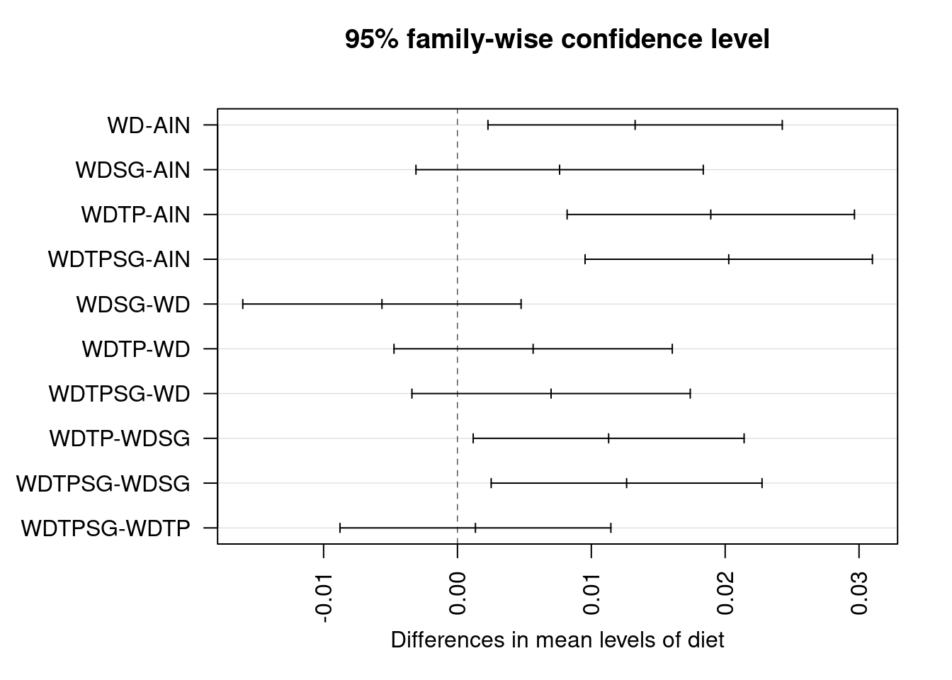

par(las = 2, mar = c(5, 8, 4, 2))
plot(TukeyHSD(adiposeaov1))

# More comprehensive method in multcomp package
par(las = 1, mar = c(5, 4, 6, 2))
library(multcomp)
library(RColorBrewer)
tuk <- glht(adiposeaov1, linfct = mcp(diet = 'Tukey'))
means <- aggregate(adipose ~ diet, adipose_weights, mean)
plot(cld(tuk, level = .05), col = brewer.pal(8, 'Pastel1'))
points(means, pch = 23)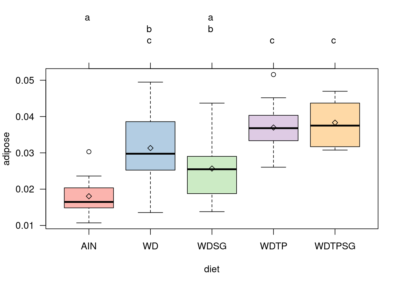

Test assumptions

plot(adiposeaov1)

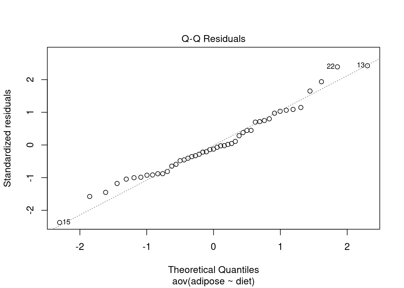
Normality

# Shapiro-Wilk W test
shapiro.test(rstandard(adiposeaov1))

## 
##  Shapiro-Wilk normality test
## 
## data:  rstandard(adiposeaov1)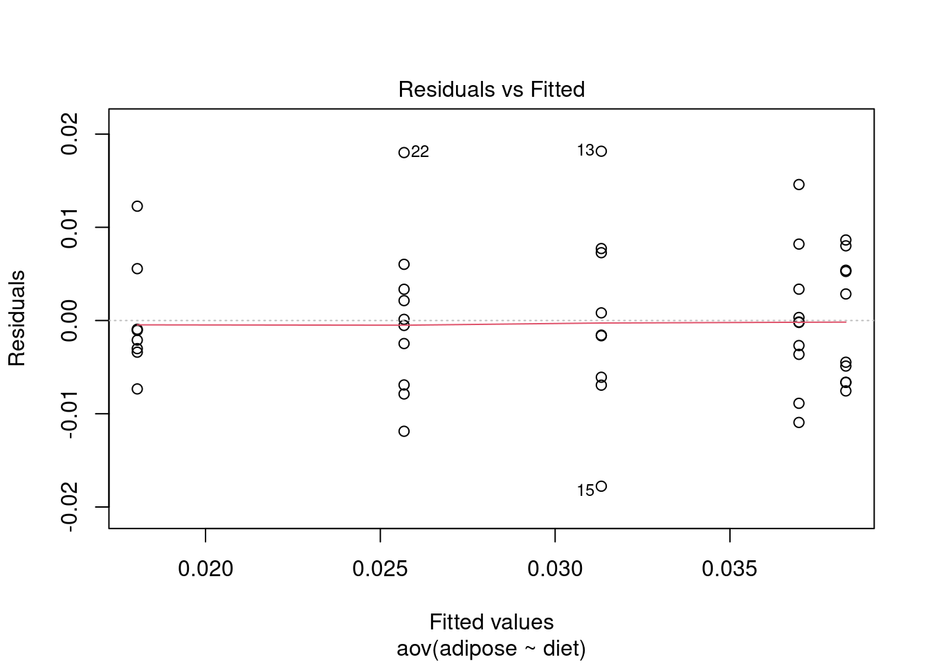
## W = 0.97688, p-value = 0.4704

Equality of variances

library(car)
leveneTest(adipose_weights$adipose, adipose_weights$diet)

## Levene's Test for Homogeneity of Variance (center = median)
##       Df F value Pr(>F)
## group  4  0.5104 0.7284
##       42

Perform ANOVA in lm for comparison

adiposelm1 <- lm(adipose_weights$adipose ~ adipose_weights$diet)
anova(adiposelm1)

## Analysis of Variance Table
## 
## Response: adipose_weights$adipose
##                      Df    Sum Sq    Mean Sq F value    Pr(>F)    
## adipose_weights$diet  4 0.0025086 0.00062714  9.9489 9.349e-06 ***
## Residuals            42 0.0026475 0.00006304                      
## ---
## Signif. codes:  0 '***' 0.001 '**' 0.01 '*' 0.05 '.' 0.1 ' ' 1

Perform regression diagnostics and test assumptions

library(gvlma)
adiposegvlmalm1 <- gvlma(adiposelm1)
summary(adiposegvlmalm1)

## 
## Call:
## lm(formula = adipose_weights$adipose ~ adipose_weights$diet)
## 
## Residuals:
##        Min         1Q     Median         3Q        Max 
## -0.0177688 -0.0054835 -0.0009354  0.0053295  0.0181588 
## 
## Coefficients:
##                            Estimate Std. Error t value Pr(>|t|)    
## (Intercept)                0.018048   0.002807   6.430 9.57e-08 ***
## adipose_weights$dietWD     0.013272   0.003858   3.440  0.00133 ** 
## adipose_weights$dietWDSG   0.007630   0.003766   2.026  0.04914 *  
## adipose_weights$dietWDTP   0.018925   0.003766   5.025 9.81e-06 ***
## adipose_weights$dietWDTPSG 0.020267   0.003766   5.381 3.06e-06 ***
## ---
## Signif. codes:  0 '***' 0.001 '**' 0.01 '*' 0.05 '.' 0.1 ' ' 1
## 
## Residual standard error: 0.00794 on 42 degrees of freedom
##   (2 observations deleted due to missingness)
## Multiple R-squared:  0.4865, Adjusted R-squared:  0.4376 
## F-statistic: 9.949 on 4 and 42 DF,  p-value: 9.349e-06
## 
## 
## ASSESSMENT OF THE LINEAR MODEL ASSUMPTIONS
## USING THE GLOBAL TEST ON 4 DEGREES-OF-FREEDOM:
## Level of Significance =  0.05 
## 
## Call:
##  gvlma(x = adiposelm1) 
## 
##                        Value p-value                Decision
## Global Stat        1.372e+00  0.8491 Assumptions acceptable.
## Skewness           1.174e+00  0.2786 Assumptions acceptable.
## Kurtosis           3.779e-02  0.8459 Assumptions acceptable.
## Link Function      3.133e-15  1.0000 Assumptions acceptable.
## Heteroscedasticity 1.598e-01  0.6893 Assumptions acceptable.

shapiro.test(rstandard(adiposelm1))

## 
##  Shapiro-Wilk normality test
## 
## data:  rstandard(adiposelm1)
## W = 0.97688, p-value = 0.4704

cor.test(fitted(adiposelm1), abs(rstandard(adiposelm1)), method = 'spearman')

## Warning in cor.test.default(fitted(adiposelm1), abs(rstandard(adiposelm1)), :
## Cannot compute exact p-value with ties

## 
##  Spearman's rank correlation rho
## 
## data:  fitted(adiposelm1) and abs(rstandard(adiposelm1))
## S = 14364, p-value = 0.2547
## alternative hypothesis: true rho is not equal to 0
## sample estimates:
##       rho 
## 0.1695033

library(car)
durbinWatsonTest(adiposelm1)

##  lag Autocorrelation D-W Statistic p-value
##    1      -0.1135751      2.212731   0.854
##  Alternative hypothesis: rho != 0

outlierTest(adiposelm1)

## No Studentized residuals with Bonferroni p < 0.05
## Largest |rstudent|:
##    rstudent unadjusted p-value Bonferroni p
## 13 2.584726           0.013403      0.62992

leveneTest(adipose_weights$adipose, adipose_weights$diet)

## Levene's Test for Homogeneity of Variance (center = median)
##       Df F value Pr(>F)
## group  4  0.5104 0.7284
##       42

Two-way factorial ANOVA example

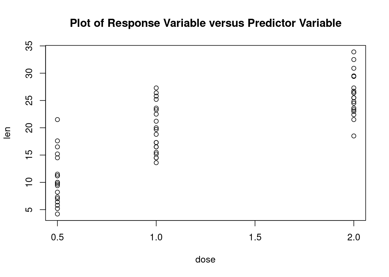
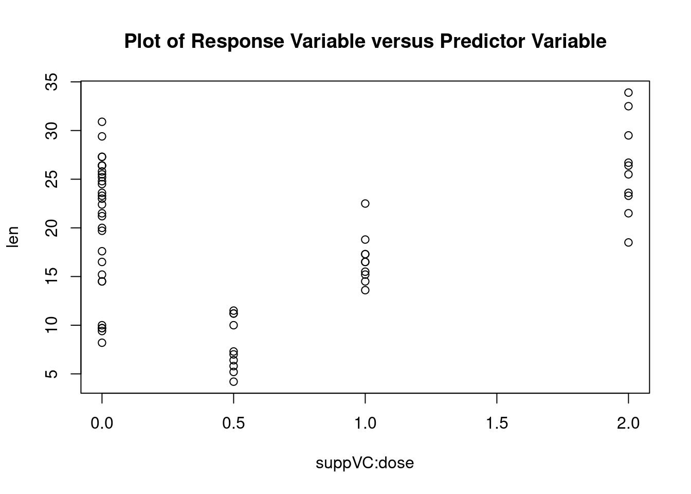
R in Action 9.5, ToothGrowth dataset

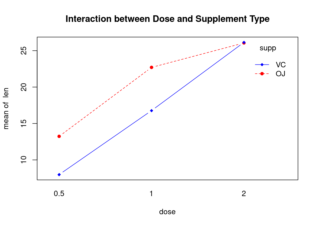
This example uses the ToothGrowth dataset in the base installation to demonstrate a two-way between-groups ANOVA. Sixty guinea pigs are randomly assigned to receive one of three levels of ascorbic acid (0.5, 1, or 2mg), and one of two delivery methods (orange juice or Vitamin C), under the restriction that each treatment combination has 10 guinea pigs. The dependent variable is tooth length.

Load dataset

attach(ToothGrowth)
table(supp, dose)

##     dose
## supp 0.5  1  2
##   OJ  10 10 10
##   VC  10 10 10

aggregate(len, by = list(supp, dose), FUN = mean)

##   Group.1 Group.2     x
## 1      OJ     0.5 13.23
## 2      VC     0.5  7.98
## 3      OJ     1.0 22.70
## 4      VC     1.0 16.77
## 5      OJ     2.0 26.06
## 6      VC     2.0 26.14

aggregate(len, by = list(supp, dose), FUN = sd)

##   Group.1 Group.2        x
## 1      OJ     0.5 4.459709
## 2      VC     0.5 2.746634
## 3      OJ     1.0 3.910953
## 4      VC     1.0 2.515309
## 5      OJ     2.0 2.655058
## 6      VC     2.0 4.797731

Perform factorial analysis of variance

fit <- lm(len ~ supp * dose)
anova(fit)

## Analysis of Variance Table
## 
## Response: len
##           Df  Sum Sq Mean Sq  F value    Pr(>F)    
## supp       1  205.35  205.35  12.3170 0.0008936 ***
## dose       1 2224.30 2224.30 133.4151 < 2.2e-16 ***
## supp:dose  1   88.92   88.92   5.3335 0.0246314 *  
## Residuals 56  933.63   16.67                       
## ---
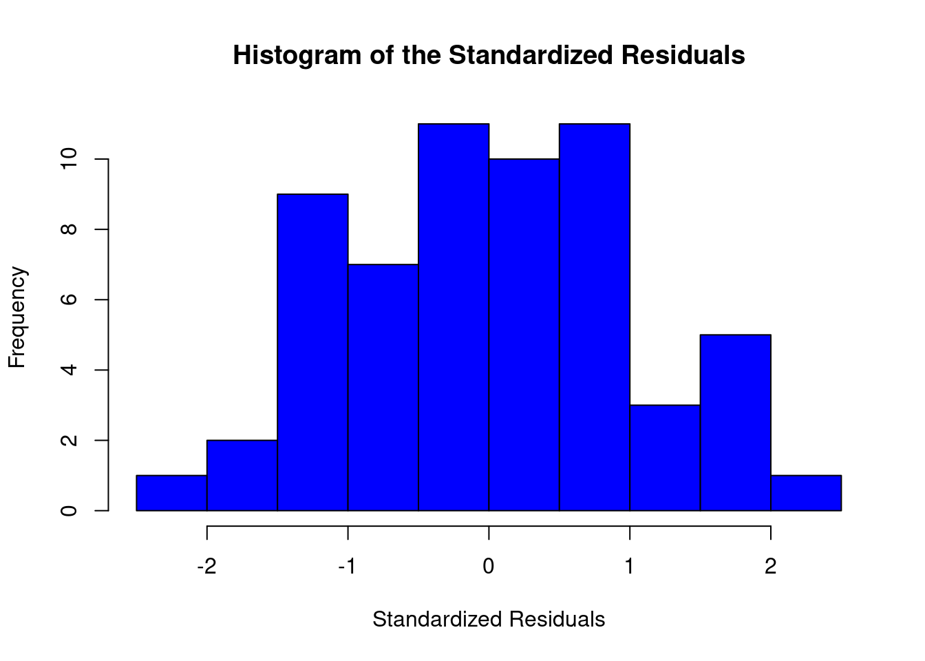
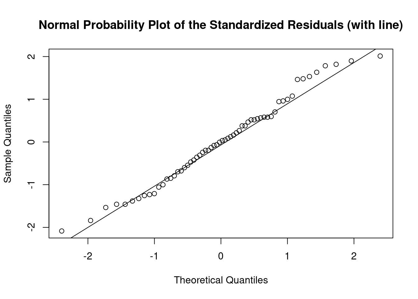
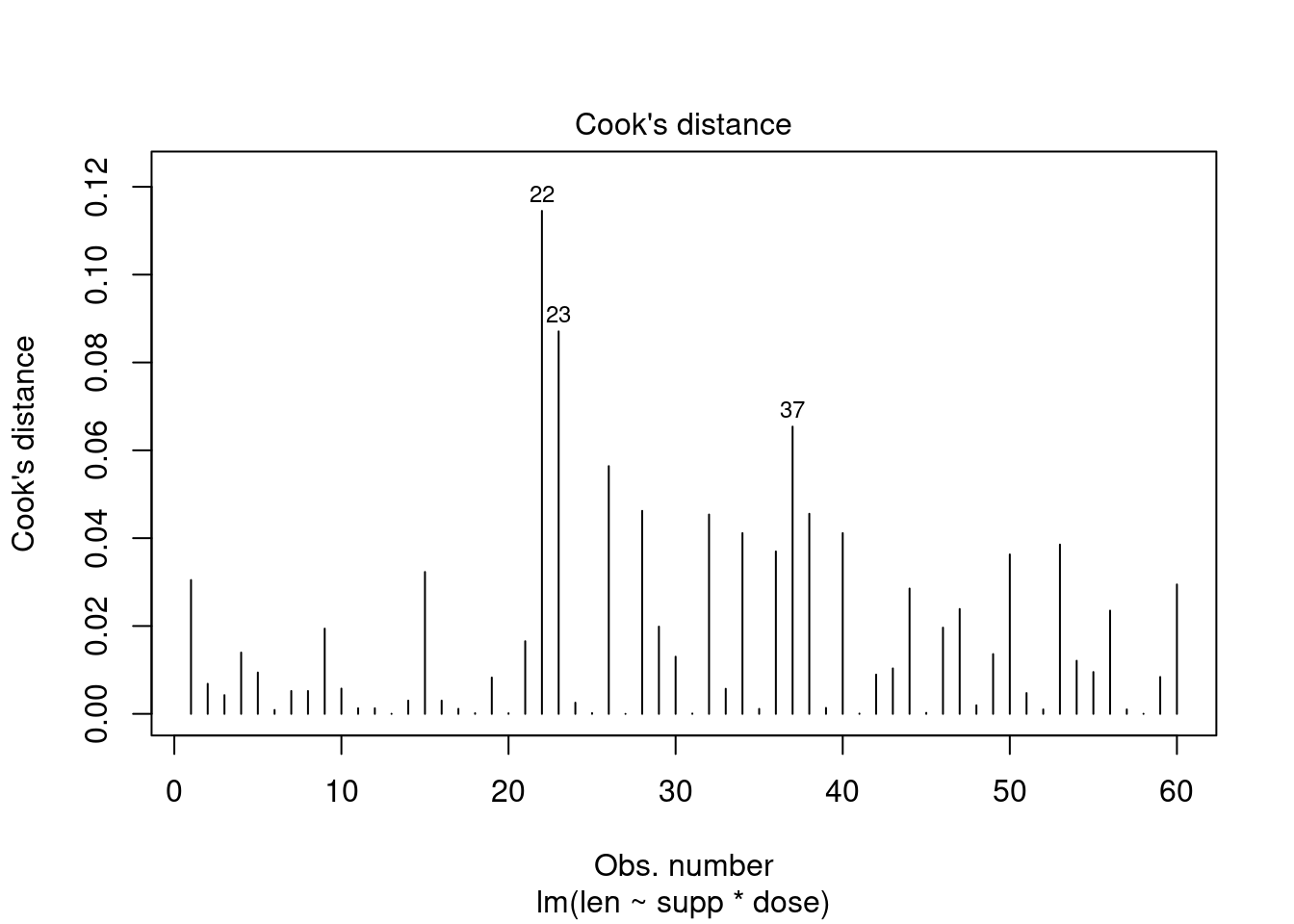
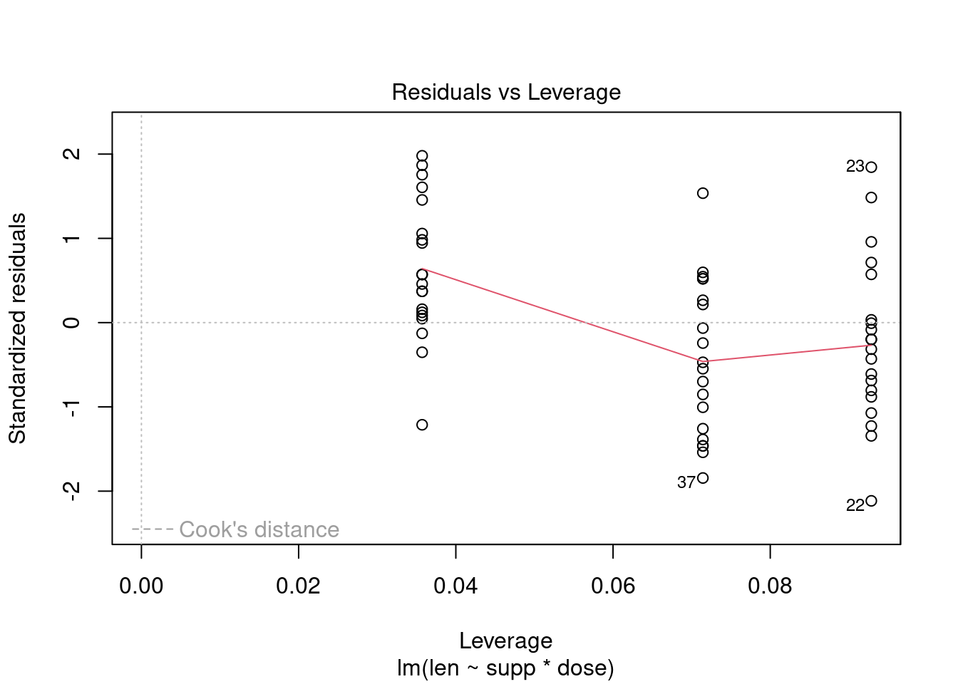
## Signif. codes:  0 '***' 0.001 '**' 0.01 '*' 0.05 '.' 0.1 ' ' 1

Perform regression diagnostics and test assumptions

library(gvlma)
gvlmafit <- gvlma(fit)
summary(gvlmafit)

## 
## Call:
## lm(formula = len ~ supp * dose)
## 
## Residuals:
##     Min      1Q  Median      3Q     Max 
## -8.2264 -2.8462  0.0504  2.2893  7.9386 
## 
## Coefficients:
##             Estimate Std. Error t value Pr(>|t|)    
## (Intercept)   11.550      1.581   7.304 1.09e-09 ***
## suppVC        -8.255      2.236  -3.691 0.000507 ***
## dose           7.811      1.195   6.534 2.03e-08 ***
## suppVC:dose    3.904      1.691   2.309 0.024631 *  
## ---
## Signif. codes:  0 '***' 0.001 '**' 0.01 '*' 0.05 '.' 0.1 ' ' 1
## 
## Residual standard error: 4.083 on 56 degrees of freedom
## Multiple R-squared:  0.7296, Adjusted R-squared:  0.7151 
## F-statistic: 50.36 on 3 and 56 DF,  p-value: 6.521e-16
## 
## 
## ASSESSMENT OF THE LINEAR MODEL ASSUMPTIONS
## USING THE GLOBAL TEST ON 4 DEGREES-OF-FREEDOM:
## Level of Significance =  0.05 
## 
## Call:
##  gvlma(x = fit) 
## 
##                      Value  p-value                   Decision
## Global Stat        10.6646 0.030604 Assumptions NOT satisfied!
## Skewness            0.0934 0.759902    Assumptions acceptable.
## Kurtosis            1.0752 0.299778    Assumptions acceptable.
## Link Function       8.7812 0.003043 Assumptions NOT satisfied!
## Heteroscedasticity  0.7148 0.397854    Assumptions acceptable.

shapiro.test(rstandard(fit))

## 
##  Shapiro-Wilk normality test
## 
## data:  rstandard(fit)
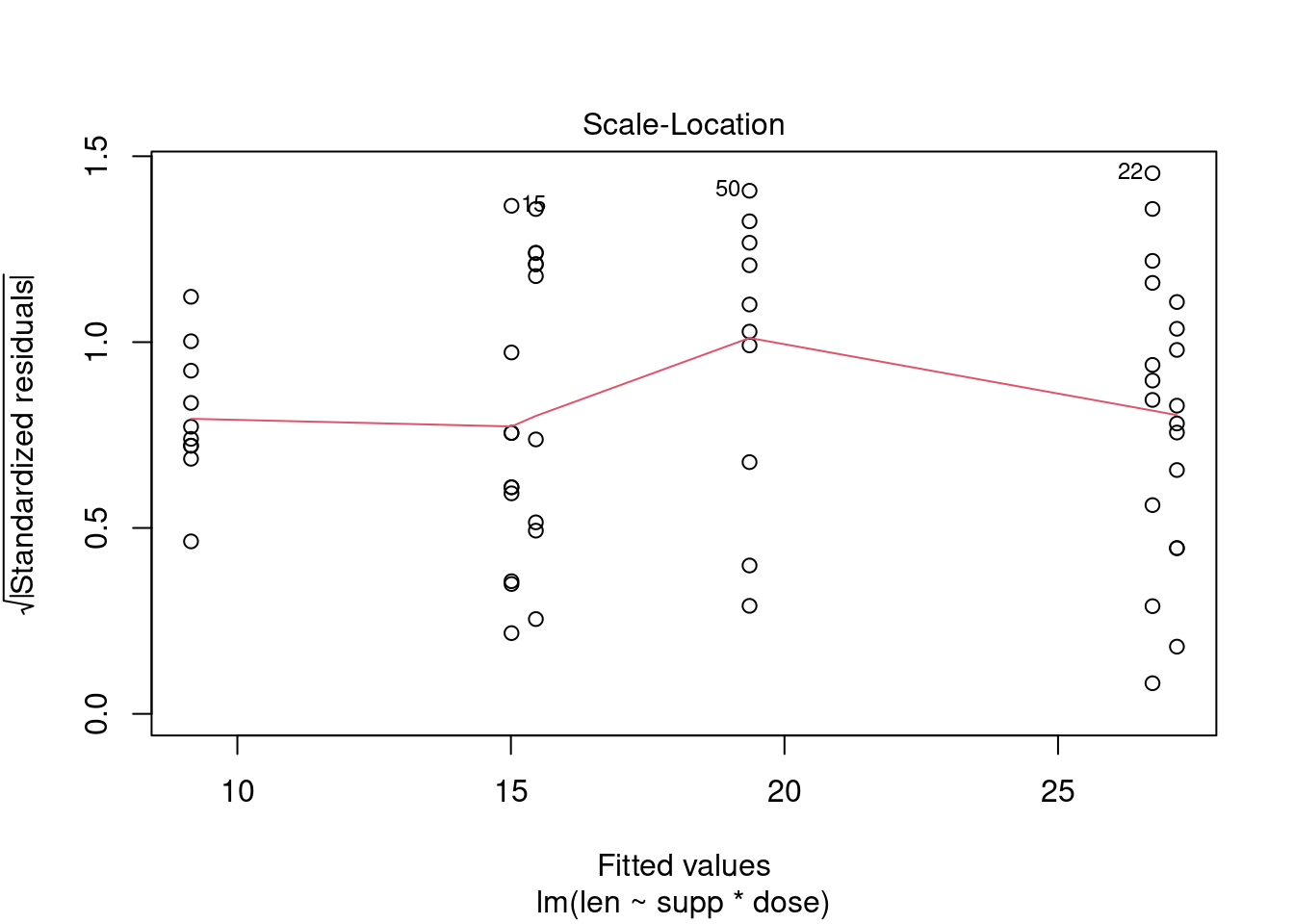
## W = 0.98147, p-value = 0.4936

cor.test(fitted(fit), abs(rstandard(fit)), method = 'spearman')

## Warning in cor.test.default(fitted(fit), abs(rstandard(fit)), method =
## "spearman"): Cannot compute exact p-value with ties

## 
##  Spearman's rank correlation rho
## 
## data:  fitted(fit) and abs(rstandard(fit))
## S = 35096, p-value = 0.8506
## alternative hypothesis: true rho is not equal to 0
## sample estimates:
##        rho 
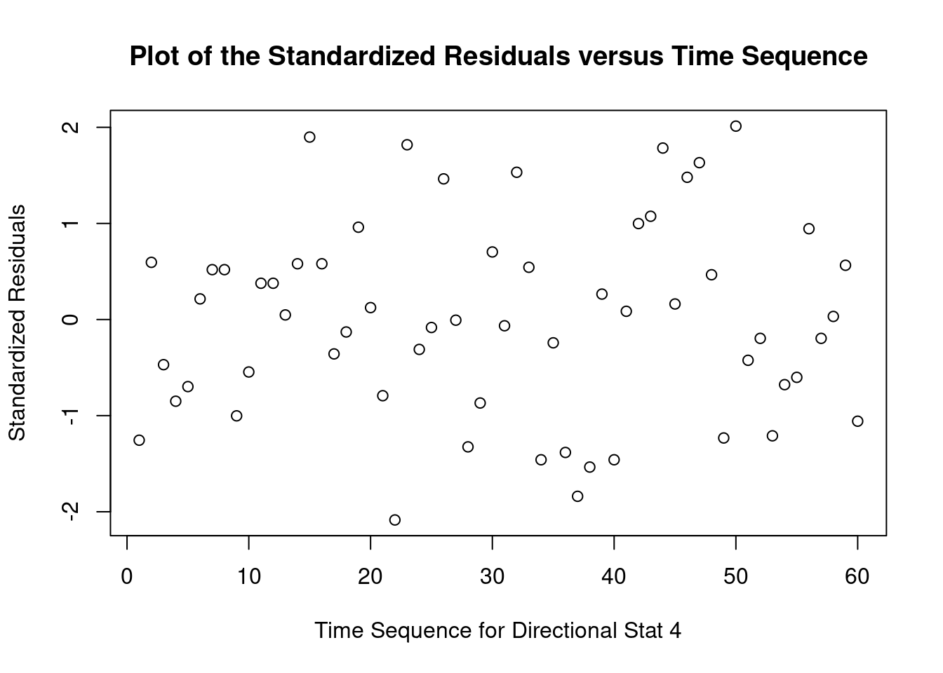
## 0.02483306

library(car)
durbinWatsonTest(fit)

##  lag Autocorrelation D-W Statistic p-value
##    1       0.1333076       1.68846   0.106
##  Alternative hypothesis: rho != 0

outlierTest(fit)

## No Studentized residuals with Bonferroni p < 0.05
## Largest |rstudent|:
##     rstudent unadjusted p-value Bonferroni p
## 22 -2.185495           0.033129           NA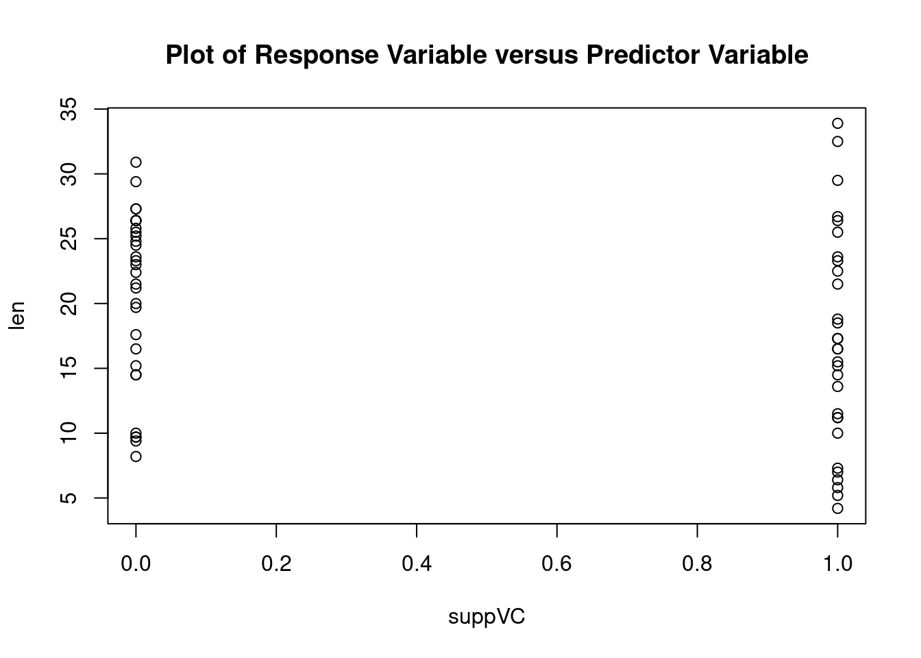

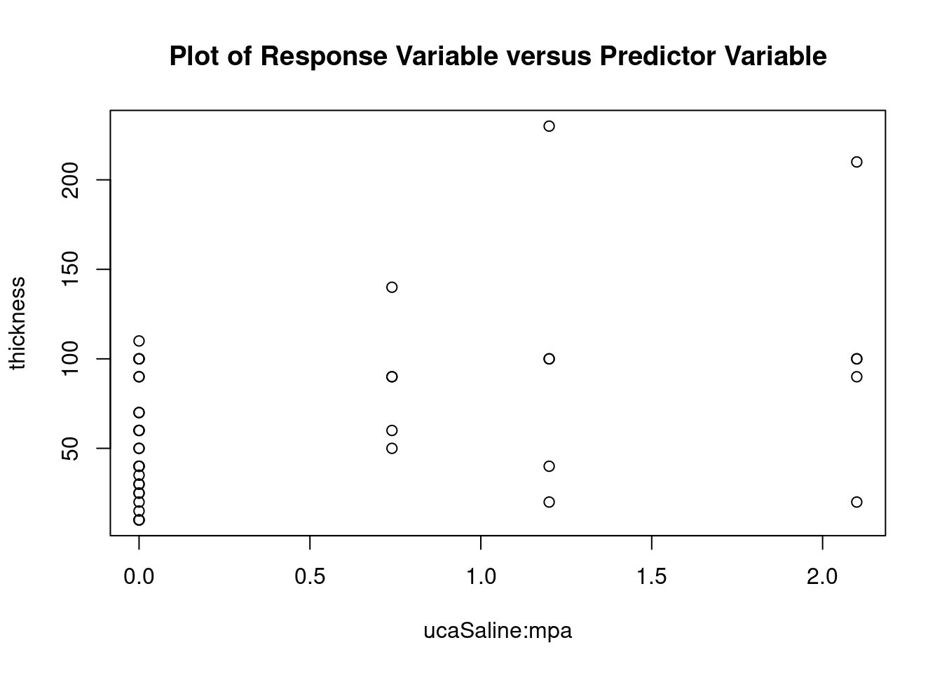
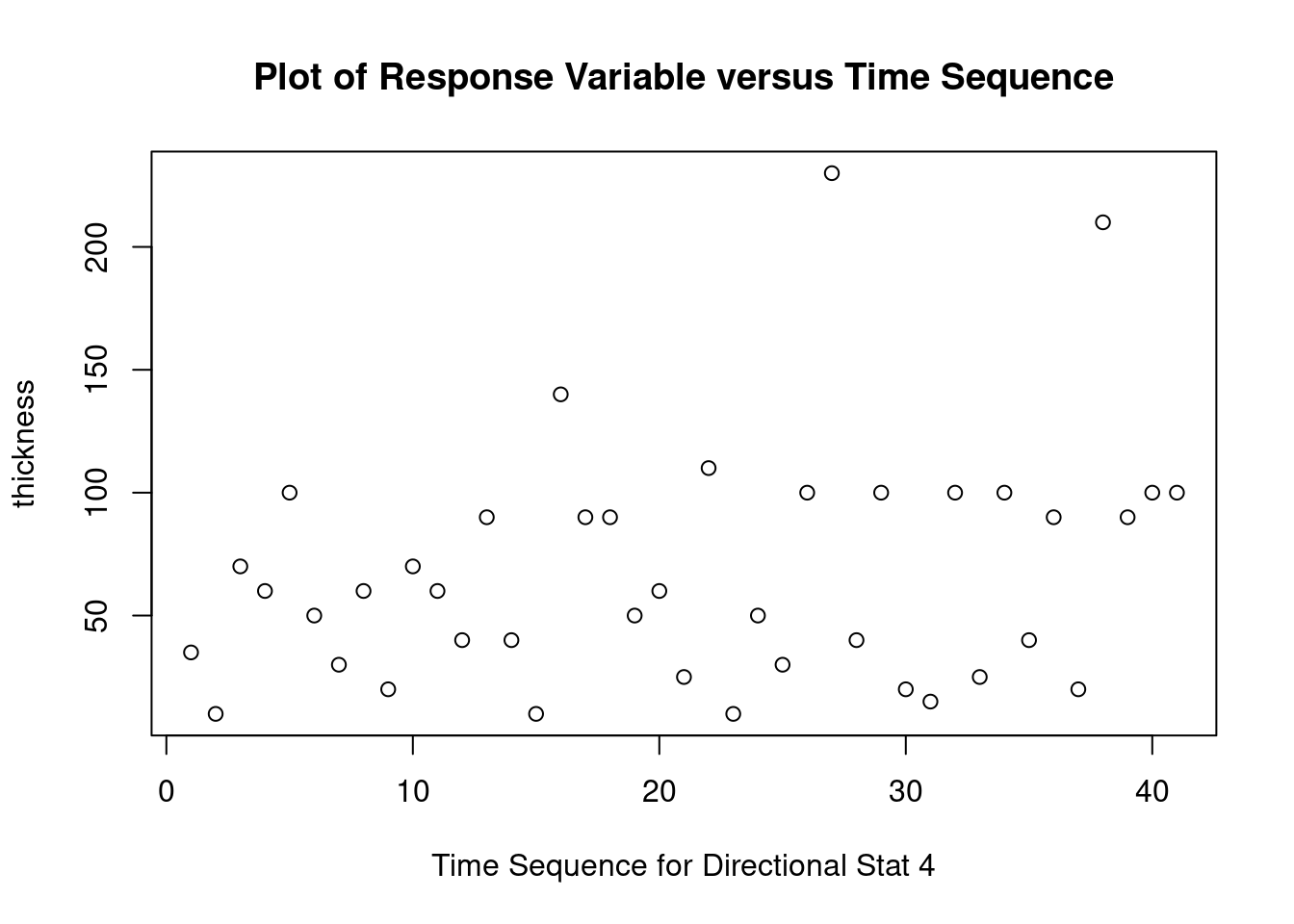
Generate plots

plot(gvlmafit, onepage = FALSE)

plot(fit, which = 3:5)

interaction.plot(
  dose,
  supp,
  len,
  type = 'b',
  col = c('red', 'blue'),
  pch = c(16, 18),
  main = 'Interaction between Dose and Supplement Type'
)

Two-way factorial ANOVA example

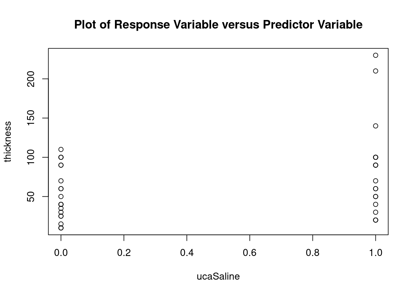
Atheroma thickness data from Smith BW et al, J Ultrasound Med 2012 (doi: 10.7863/jum.2012.31.5.711).

Import dataset

fall2009thickness <-
  read.table(
    'data/anova_factorial_jum2012_atheroma_thickness.csv',
    header = TRUE,
    sep = ','
  )
attach(fall2009thickness)
head(fall2009thickness)

##     id      uca mpa thickness
## 1 L604 Definity   0        35
## 2 L611 Definity   0        10
## 3 L614 Definity   0        70
## 4 L617 Definity   0        60
## 5 L624 Definity   0       100
## 6 L593   Saline   0        50

Perform factorial analysis of variance

thick_fit <- lm(thickness ~ uca * mpa, data = fall2009thickness)
anova(thick_fit)

## Analysis of Variance Table
## 
## Response: thickness
##           Df Sum Sq Mean Sq F value  Pr(>F)  
## uca        1   9619  9618.9  4.6436 0.03775 *
## mpa        1   5255  5255.4  2.5371 0.11971  
## uca:mpa    1   3285  3285.1  1.5859 0.21580  
## Residuals 37  76643  2071.4                  
## ---
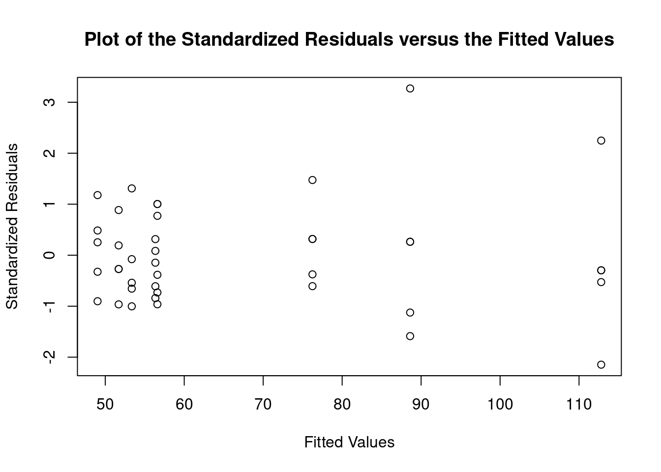
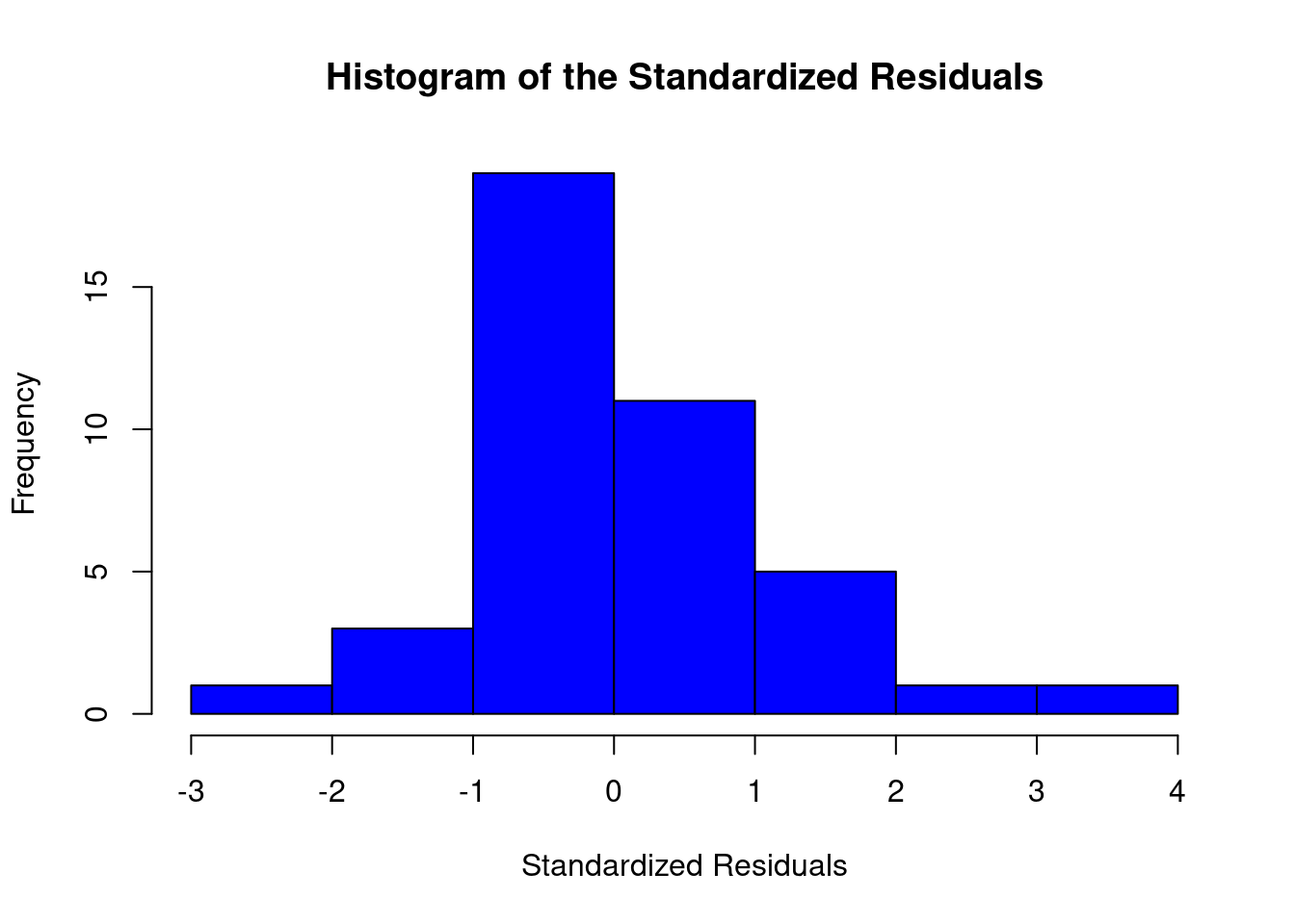
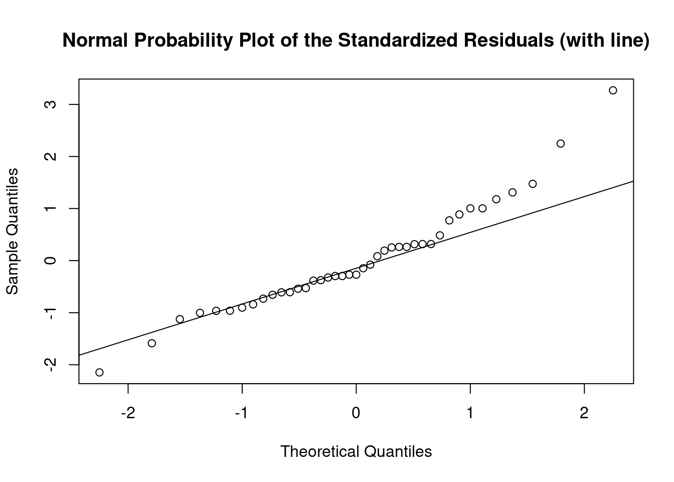
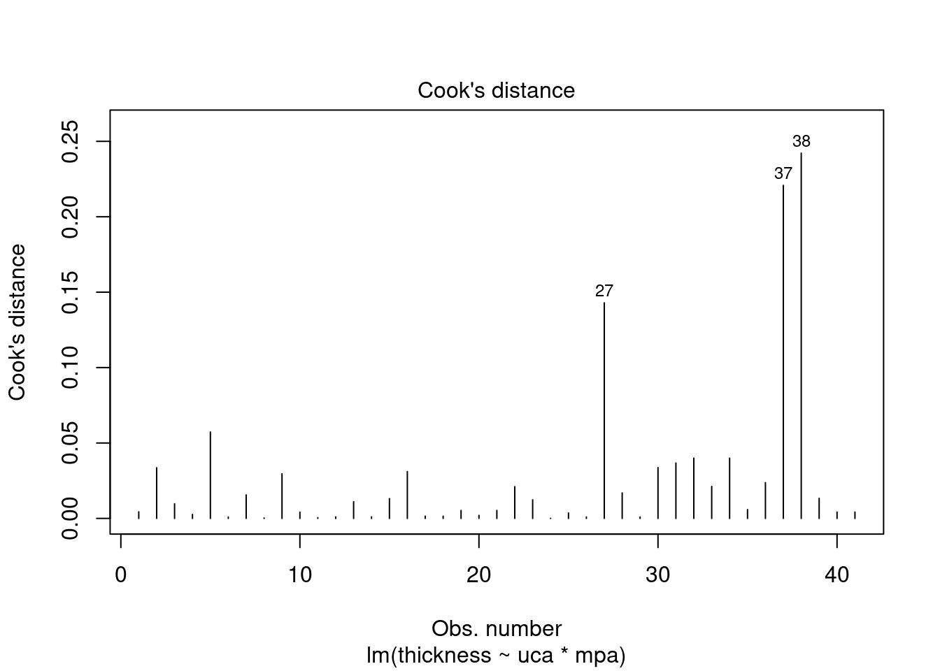
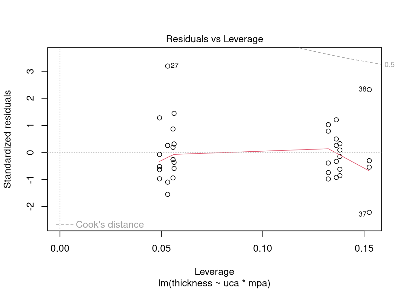
## Signif. codes:  0 '***' 0.001 '**' 0.01 '*' 0.05 '.' 0.1 ' ' 1

Perform regression diagnostics and test assumptions

library(gvlma)
gvlmathick_fit <- gvlma(thick_fit)
summary(gvlmathick_fit)

## 
## Call:
## lm(formula = thickness ~ uca * mpa, data = fall2009thickness)
## 
## Residuals:
##    Min     1Q Median     3Q    Max 
## -92.81 -26.34 -11.70  13.76 141.39 
## 
## Coefficients:
##               Estimate Std. Error t value Pr(>|t|)   
## (Intercept)     49.026     16.802   2.918  0.00596 **
## ucaSaline        7.320     23.838   0.307  0.76053   
## mpa              3.608     12.762   0.283  0.77898   
## ucaSaline:mpa   23.278     18.484   1.259  0.21580   
## ---
## Signif. codes:  0 '***' 0.001 '**' 0.01 '*' 0.05 '.' 0.1 ' ' 1
## 
## Residual standard error: 45.51 on 37 degrees of freedom
## Multiple R-squared:  0.1915, Adjusted R-squared:  0.126 
## F-statistic: 2.922 on 3 and 37 DF,  p-value: 0.04662
## 
## 
## ASSESSMENT OF THE LINEAR MODEL ASSUMPTIONS
## USING THE GLOBAL TEST ON 4 DEGREES-OF-FREEDOM:
## Level of Significance =  0.05 
## 
## Call:
##  gvlma(x = thick_fit) 
## 
##                      Value  p-value                   Decision
## Global Stat        15.0581 0.004582 Assumptions NOT satisfied!
## Skewness            5.2041 0.022534 Assumptions NOT satisfied!
## Kurtosis            4.1197 0.042388 Assumptions NOT satisfied!
## Link Function       0.9562 0.328138    Assumptions acceptable.
## Heteroscedasticity  4.7782 0.028823 Assumptions NOT satisfied!

shapiro.test(rstandard(thick_fit))

## 
##  Shapiro-Wilk normality test
## 
## data:  rstandard(thick_fit)
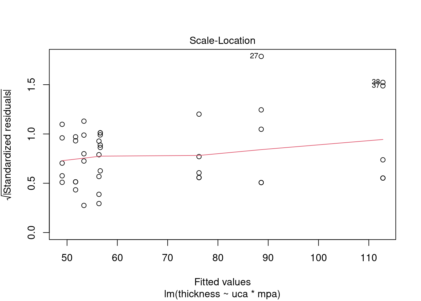
## W = 0.95015, p-value = 0.07084

cor.test(fitted(thick_fit), abs(rstandard(thick_fit)), method = 'spearman')

## Warning in cor.test.default(fitted(thick_fit), abs(rstandard(thick_fit)), :
## Cannot compute exact p-value with ties

## 
##  Spearman's rank correlation rho
## 
## data:  fitted(thick_fit) and abs(rstandard(thick_fit))
## S = 9194.5, p-value = 0.2121
## alternative hypothesis: true rho is not equal to 0
## sample estimates:
##      rho 
## 0.199083

library(car)
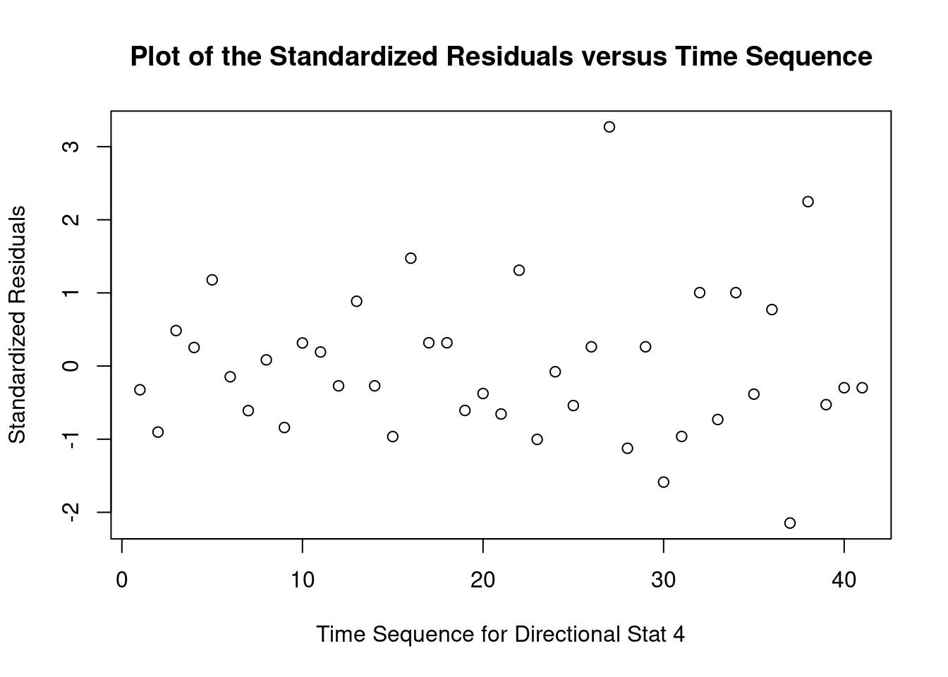
durbinWatsonTest(thick_fit)

##  lag Autocorrelation D-W Statistic p-value
##    1      -0.3832382       2.76177    0.03
##  Alternative hypothesis: rho != 0

outlierTest(thick_fit)

##    rstudent unadjusted p-value Bonferroni p
## 27 3.699668         0.00071694     0.029395

Generate plots

plot(gvlmathick_fit, onepage = FALSE)

plot(thick_fit, which = 3:5)

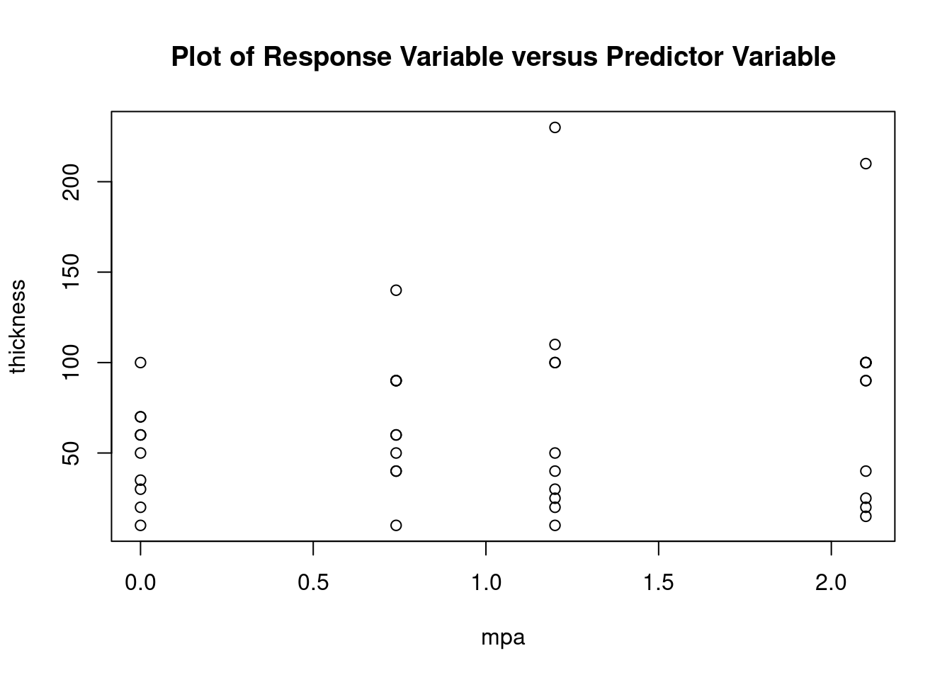
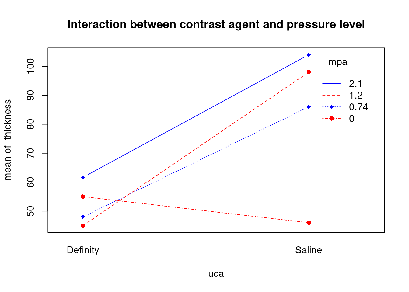
interaction.plot(
  uca,
  mpa,
  thickness,
  type = 'b',
  col = c('red', 'blue'),
  pch = c(16, 18),
  main = 'Interaction between contrast agent and pressure level'
)

Log transform to correct non-normality, heteroscedasticity, and outlier

log_thick_fit <- lm(log(thickness) ~ uca * mpa, data = fall2009thickness)
anova(log_thick_fit)

## Analysis of Variance Table
## 
## Response: log(thickness)
##           Df  Sum Sq Mean Sq F value  Pr(>F)  
## uca        1  2.4372 2.43722  4.1806 0.04805 *
## mpa        1  0.6951 0.69511  1.1923 0.28192  
## uca:mpa    1  0.3084 0.30843  0.5291 0.47158  
## Residuals 37 21.5703 0.58298                  
## ---
## Signif. codes:  0 '***' 0.001 '**' 0.01 '*' 0.05 '.' 0.1 ' ' 1

Perform regression diagnostics and test assumptions

library(gvlma)
gvlma_log_thick_fit <- gvlma(log_thick_fit)
summary(gvlma_log_thick_fit)

## 
## Call:
## lm(formula = log(thickness) ~ uca * mpa, data = fall2009thickness)
## 
## Residuals:
##      Min       1Q   Median       3Q      Max 
## -1.51653 -0.50113  0.09291  0.44825  1.18425 
## 
## Coefficients:
##               Estimate Std. Error t value Pr(>|t|)    
## (Intercept)    3.64610    0.28187  12.935 2.67e-15 ***
## ucaSaline      0.26316    0.39991   0.658    0.515    
## mpa            0.06159    0.21410   0.288    0.775    
## ucaSaline:mpa  0.22555    0.31009   0.727    0.472    
## ---
## Signif. codes:  0 '***' 0.001 '**' 0.01 '*' 0.05 '.' 0.1 ' ' 1
## 
## Residual standard error: 0.7635 on 37 degrees of freedom
## Multiple R-squared:  0.1376, Adjusted R-squared:  0.06764 
## F-statistic: 1.967 on 3 and 37 DF,  p-value: 0.1358
## 
## 
## ASSESSMENT OF THE LINEAR MODEL ASSUMPTIONS
## USING THE GLOBAL TEST ON 4 DEGREES-OF-FREEDOM:
## Level of Significance =  0.05 
## 
## Call:
##  gvlma(x = log_thick_fit) 
## 
##                     Value p-value                Decision
## Global Stat        3.4821  0.4806 Assumptions acceptable.
## Skewness           2.1479  0.1428 Assumptions acceptable.
## Kurtosis           0.5245  0.4689 Assumptions acceptable.
## Link Function      0.6395  0.4239 Assumptions acceptable.
## Heteroscedasticity 0.1701  0.6800 Assumptions acceptable.

shapiro.test(rstandard(log_thick_fit))

## 
##  Shapiro-Wilk normality test
## 
## data:  rstandard(log_thick_fit)
## W = 0.93909, p-value = 0.02924

cor.test(fitted(log_thick_fit),
         abs(rstandard(log_thick_fit)),
         method = 'spearman')

## Warning in cor.test.default(fitted(log_thick_fit),
## abs(rstandard(log_thick_fit)), : Cannot compute exact p-value with ties

## 
##  Spearman's rank correlation rho
## 
## data:  fitted(log_thick_fit) and abs(rstandard(log_thick_fit))
## S = 12485, p-value = 0.5861
## alternative hypothesis: true rho is not equal to 0
## sample estimates:
##         rho 
## -0.08758111

library(car)
durbinWatsonTest(log_thick_fit)

##  lag Autocorrelation D-W Statistic p-value
##    1      -0.3411439      2.681506    0.08
##  Alternative hypothesis: rho != 0

outlierTest(log_thick_fit)

## No Studentized residuals with Bonferroni p < 0.05
## Largest |rstudent|:
##     rstudent unadjusted p-value Bonferroni p
## 37 -2.276215           0.028882           NA

Generate plots

plot(gvlma_log_thick_fit, onepage = FALSE)

plot(log_thick_fit, which = 3:5)

interaction.plot(
  uca,
  mpa,
  thickness,
  type = 'b',
  col = c('red', 'blue'),
  pch = c(16, 18),
  main = 'Interaction between contrast agent and pressure level'
)

ANOVA Compact Letter Display

Compact Letter Display (CLD) for ANOVA multiple comparisons with the multcomp package

# multiple comparison procedures
# set up a one-way ANOVA
library(multcomp)
data(warpbreaks)
amod <- aov(breaks ~ tension, data = warpbreaks)
# specify all pair-wise comparisons among levels of variable 'tension'
tuk <- glht(amod, linfct = mcp(tension = 'Tukey'))
# extract information
tuk.cld <- cld(tuk)
# use sufficiently large upper margin
old.par <- par(mai = c(1, 1, 1.5, 1))
# plot
plot(tuk.cld)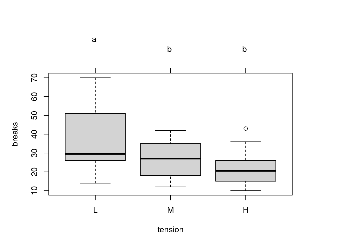

par(old.par)

Repeated measures ANOVA

Repeated measures ANOVA example

R in Action 2nd ed, 9.6, CO2 dataset

note that the code from the first edition may return errors

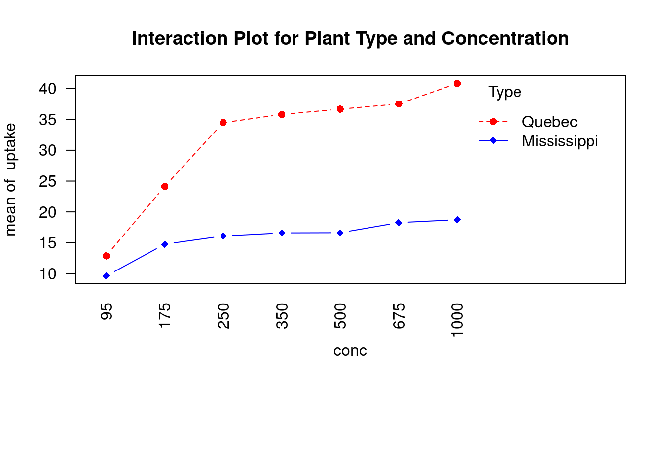
In addition to the base installation, we’ll be using the car, gplots, HH, rrcov, and mvoutlier packages in our examples. Be sure to install them before trying out the sample code.

The CO2 dataset included in the base installation contains the results of a study of cold tolerance in Northern and Southern plants of the grass species Echinochloa crus-galli (Potvin, Lechowicz, & Tardif, 1990). The photosynthetic rates of chilled plants were compared with the photosynthetic rates of nonchilled plants at several ambient CO2 concentrations. Half the plants were from Quebec, and half were from Mississippi.

In this example, we’ll focus on chilled plants. The dependent variable is carbon dioxide uptake (uptake) in ml/L, and the independent variables are Type (Quebec versus Mississippi) and ambient CO2 concentration (conc) with seven levels (ranging from 95 to 1000 umol/m^2 sec). Type is a between-groups factor, and conc is a within- groups factor. Type is already stored as a factor, but you’ll need to convert conc to a factor before continuing. The analysis is presented in the next listing.

CO2$conc <- factor(CO2$conc)
w1b1 <- subset(CO2, Treatment == 'chilled')
co2_fit <- aov(uptake ~ conc * Type + Error(Plant / (conc)), w1b1)
summary(co2_fit)

## 
## Error: Plant
##           Df Sum Sq Mean Sq F value  Pr(>F)   
## Type       1 2667.2  2667.2   60.41 0.00148 **
## Residuals  4  176.6    44.1                   
## ---
## Signif. codes:  0 '***' 0.001 '**' 0.01 '*' 0.05 '.' 0.1 ' ' 1
## 
## Error: Plant:conc
##           Df Sum Sq Mean Sq F value   Pr(>F)    
## conc       6 1472.4  245.40   52.52 1.26e-12 ***
## conc:Type  6  428.8   71.47   15.30 3.75e-07 ***
## Residuals 24  112.1    4.67                     
## ---
## Signif. codes:  0 '***' 0.001 '**' 0.01 '*' 0.05 '.' 0.1 ' ' 1

par(las = 2)
par(mar = c(10, 4, 4, 2))
with(
  w1b1,
  interaction.plot(
    conc,
    Type,
    uptake,
    type = 'b',
    col = c('red', 'blue'),
    pch = c(16, 18),
    main = 'Interaction Plot for Plant Type and Concentration'
  )
)

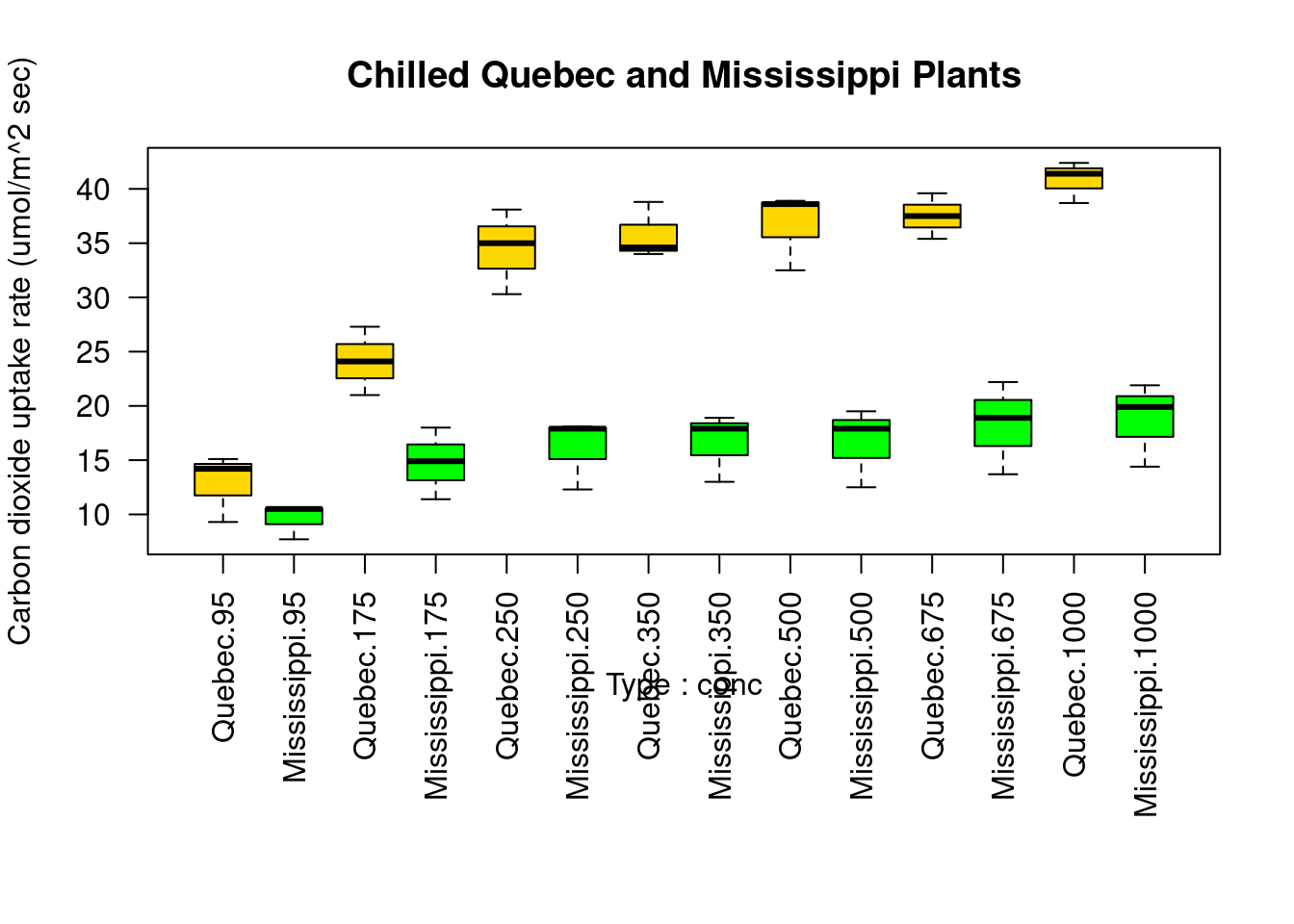
boxplot(
  uptake ~ Type * conc,
  data = w1b1,
  col = (c('gold', 'green')),
  main = 'Chilled Quebec and Mississippi Plants',
  ylab = 'Carbon dioxide uptake rate (umol/m^2 sec)'
)

The many approaches to mixed-model designs

The CO2 example in this section was analyzed using a traditional repeated measures ANOVA. The approach assumes that the covariance matrix for any within-groups factor follows a specified form known as sphericity. Specifically, it assumes that the vari- ances of the differences between any two levels of the within-groups factor are equal. In real-world data, it’s unlikely that this assumption will be met. This has led to a number of alternative approaches, including the following:

Using the lmer() function in the lme4 package to fit linear mixed models (Bates, 2005)

Using the Anova() function in the car package to adjust traditional test statis- tics to account for lack of sphericity (for example, the Geisser–Greenhouse correction)

Using the gls() function in the nlme package to fit generalized least squares models with specified variance-covariance structures (UCLA, 2009)

Using multivariate analysis of variance to model repeated measured data (Hand, 1987)

Coverage of these approaches is beyond the scope of this text. If you’re interested in learning more, check out Pinheiro and Bates (2000) and Zuur et al. (2009).

ANCOVA

One-way ANCOVA example

R in Action 9.4, litter dataset from multcomp package

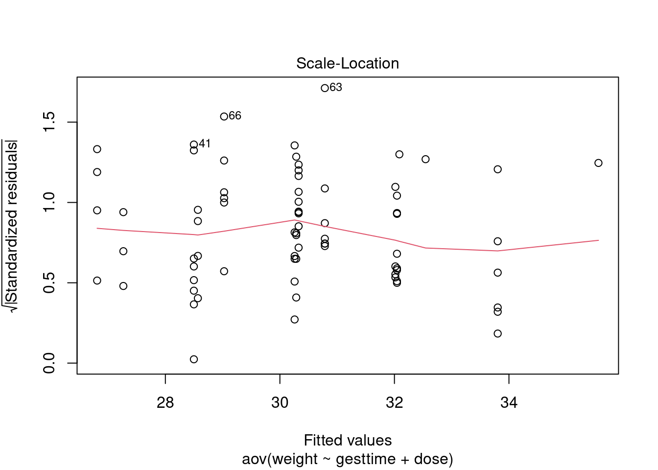
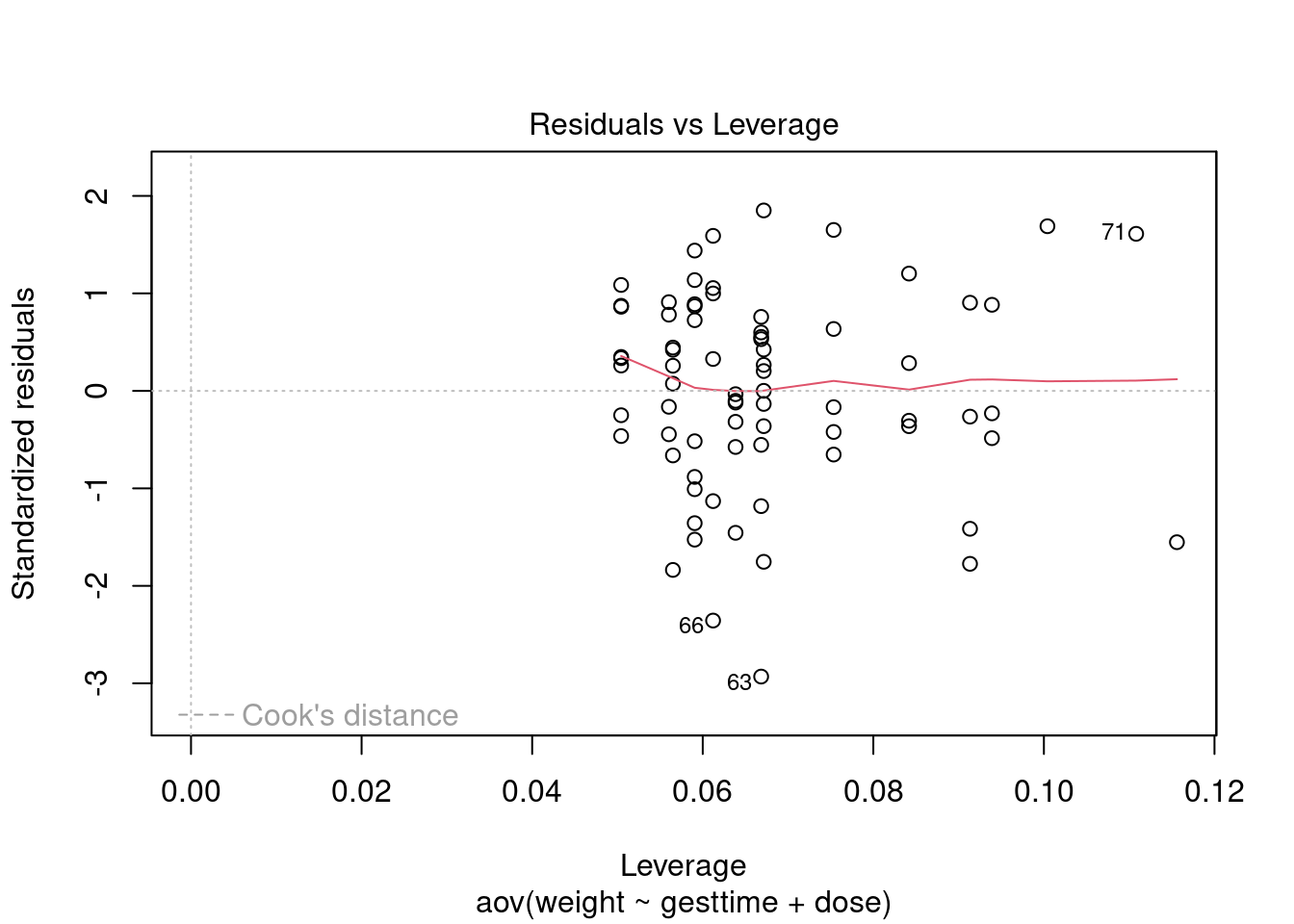
Pregnant mice were divided into four treatment groups; each group received a different dose of a drug (0, 5, 50, or 500). The mean post-birth weight for each litter was the dependent variable and gestation time was included as a covariate. The analysis is given in the following listing.

Load dataset

library(multcomp)
attach(litter)
table(dose)

## dose
##   0   5  50 500 
##  20  19  18  17

aggregate(weight, by = list(dose), FUN = mean)

##   Group.1        x
## 1       0 32.30850
## 2       5 29.30842
## 3      50 29.86611
## 4     500 29.64647

Perform analysis of covariance

litter_fit <- aov(weight ~ gesttime + dose)
summary(litter_fit)

##             Df Sum Sq Mean Sq F value  Pr(>F)   
## gesttime     1  134.3  134.30   8.049 0.00597 **
## dose         3  137.1   45.71   2.739 0.04988 * 
## Residuals   69 1151.3   16.69                   
## ---
## Signif. codes:  0 '***' 0.001 '**' 0.01 '*' 0.05 '.' 0.1 ' ' 1

Calculate adjusted group means

Because you’re using a covariate, you may want to obtain adjusted group means—that is, the group means obtained after partialing out the effects of the covariate. You can use the effect() function in the effects library to calculate adjusted means:

library(effects)

## lattice theme set by effectsTheme()
## See ?effectsTheme for details.

effect('dose', litter_fit)

## 
##  dose effect
## dose
##        0        5       50      500 
## 32.35367 28.87672 30.56614 29.33460

In this case, the adjusted means are similar to the unadjusted means produced by the aggregate() function, but this won’t always be the case. The effects package provides a powerful method of obtaining adjusted means for complex research designs and presenting them visually. See the package documentation on CRAN for more details.

Multiple comparisons

library(multcomp)
litter_contrast <- rbind('no drug vs. drug' = c(3,-1,-1,-1))
summary(glht(litter_fit, linfct = mcp(dose = litter_contrast)))

## 
##   Simultaneous Tests for General Linear Hypotheses
## 
## Multiple Comparisons of Means: User-defined Contrasts
## 
## 
## Fit: aov(formula = weight ~ gesttime + dose)
## 
## Linear Hypotheses:
##                       Estimate Std. Error t value Pr(>|t|)  
## no drug vs. drug == 0    8.284      3.209   2.581    0.012 *
## ---
## Signif. codes:  0 '***' 0.001 '**' 0.01 '*' 0.05 '.' 0.1 ' ' 1
## (Adjusted p values reported -- single-step method)

The contrast c(3, -1, -1, -1) specifies a comparison of the first group with the average of the other three. The hypothesis is tested with a t statistic (2.581 in this case), which is significant at the p < .05 level. Therefore, you can conclude that the no-drug group has a higher birth weight than drug conditions. Other contrasts can be added to the rbind() function (see help(glht) for details).

Assumptions

# global validation of linear model assumptions
library(gvlma)
gvlmalitter <- gvlma(lm(weight ~ gesttime + dose, data = litter))
summary(gvlmalitter)

## 
## Call:
## lm(formula = weight ~ gesttime + dose, data = litter)
## 
## Residuals:
##      Min       1Q   Median       3Q      Max 
## -11.5649  -2.0068   0.1476   3.0755   7.3023 
## 
## Coefficients:
##             Estimate Std. Error t value Pr(>|t|)   
## (Intercept)  -45.366     24.984  -1.816  0.07374 . 
## gesttime       3.519      1.131   3.111  0.00271 **
## dose5         -3.477      1.318  -2.639  0.01027 * 
## dose50        -1.788      1.344  -1.330  0.18780   
## dose500       -3.019      1.352  -2.232  0.02883 * 
## ---
## Signif. codes:  0 '***' 0.001 '**' 0.01 '*' 0.05 '.' 0.1 ' ' 1
## 
## Residual standard error: 4.085 on 69 degrees of freedom
## Multiple R-squared:  0.1908, Adjusted R-squared:  0.1439 
## F-statistic: 4.067 on 4 and 69 DF,  p-value: 0.005105
## 
## 
## ASSESSMENT OF THE LINEAR MODEL ASSUMPTIONS
## USING THE GLOBAL TEST ON 4 DEGREES-OF-FREEDOM:
## Level of Significance =  0.05 
## 
## Call:
##  gvlma(x = lm(weight ~ gesttime + dose, data = litter)) 
## 
##                        Value p-value                Decision
## Global Stat        8.3233466 0.08043 Assumptions acceptable.
## Skewness           3.0816555 0.07918 Assumptions acceptable.
## Kurtosis           0.0002286 0.98794 Assumptions acceptable.
## Link Function      3.3202398 0.06843 Assumptions acceptable.
## Heteroscedasticity 1.9212226 0.16572 Assumptions acceptable.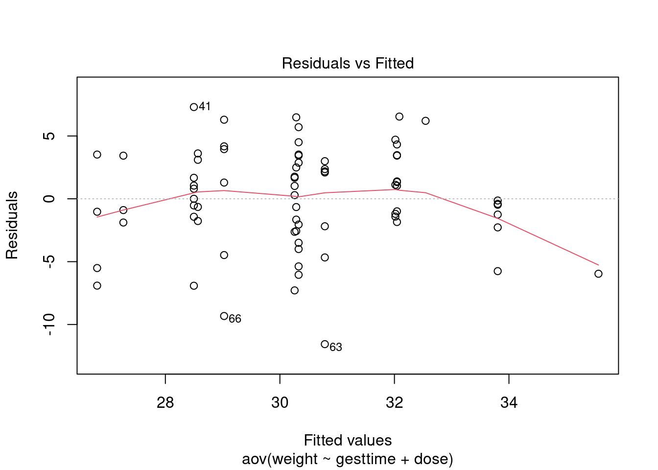

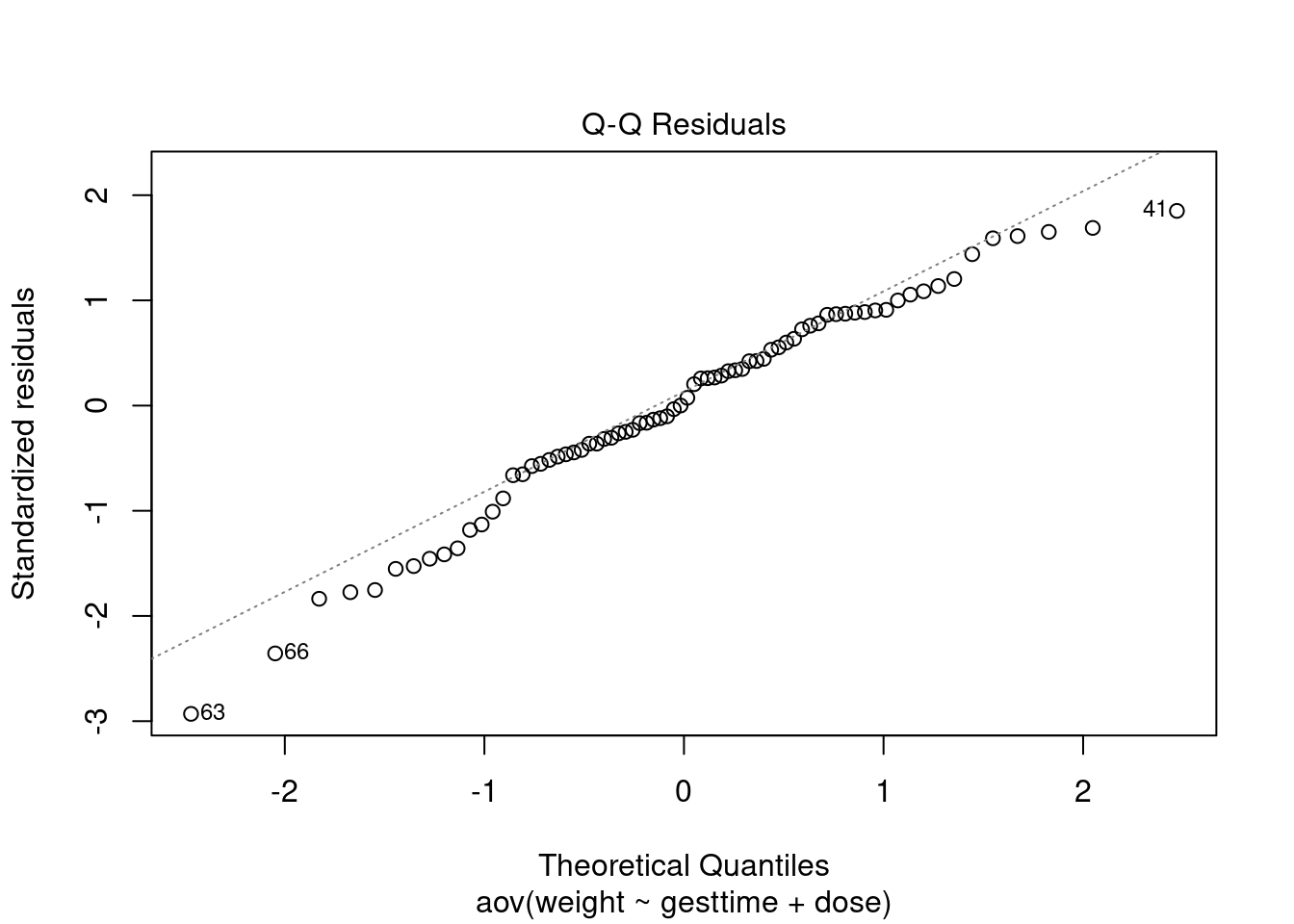
plot(litter_fit)

Normality

# Shapiro-Wilk W test
shapiro.test(rstandard(litter_fit))

## 
##  Shapiro-Wilk normality test
## 
## data:  rstandard(litter_fit)
## W = 0.97617, p-value = 0.175

Equality of variances

Note that the Brown-Forsythe test returns a significant result, indicating heterogeneity of residual variances. However, this is for a one-way model without the gesttime covariate. Including the covariate accounts for significant residual variance and satisfies all gvlma assumptions.

library(car)
leveneTest(weight, dose, data = litter)

## Levene's Test for Homogeneity of Variance (center = median: litter)
##       Df F value  Pr(>F)  
## group  3  3.1788 0.02925 *
##       70                  
## ---
## Signif. codes:  0 '***' 0.001 '**' 0.01 '*' 0.05 '.' 0.1 ' ' 1

MANOVA

MANOVA = Multivariate Analysis of Variance

MANOVA example

Ultrasound data

Import dataset

hr <- read.table('data/manova_hr.csv', header = TRUE, sep = ',')
attach(hr)
names(hr)

## [1] "US"   "USC"  "V"    "VC"   "Time"

Perform multivariate ANOVA

skull.manova1 = manova(cbind(US, USC, V, VC) ~ as.factor(Time), data = hr)
summary(skull.manova1)

##                 Df  Pillai approx F num Df den Df Pr(>F)
## as.factor(Time)  2 0.65326   1.2127      8     20 0.3412
## Residuals       12

summary(skull.manova1, test = 'Wilks')

##                 Df   Wilks approx F num Df den Df Pr(>F)
## as.factor(Time)  2 0.35085   1.5486      8     18 0.2094
## Residuals       12

summary(skull.manova1, test = 'Hotelling-Lawley')

##                 Df Hotelling-Lawley approx F num Df den Df Pr(>F)
## as.factor(Time)  2           1.8385   1.8385      8     16 0.1427
## Residuals       12

summary(skull.manova1, test = 'Roy')

##                 Df    Roy approx F num Df den Df  Pr(>F)  
## as.factor(Time)  2 1.8321   4.5803      4     10 0.02324 *
## Residuals       12                                        
## ---
## Signif. codes:  0 '***' 0.001 '**' 0.01 '*' 0.05 '.' 0.1 ' ' 1

Fisher’s exact

Fisher’s exact test arthritis example

Arthritis data from vcd package

Load dataset

# see R in Action section 7.2 for walkthrough
library(vcd)

## Loading required package: grid

summary(Arthritis)

##        ID          Treatment      Sex          Age          Improved 
##  Min.   : 1.00   Placebo:43   Female:59   Min.   :23.00   None  :42  
##  1st Qu.:21.75   Treated:41   Male  :25   1st Qu.:46.00   Some  :14  
##  Median :42.50                            Median :57.00   Marked:28  
##  Mean   :42.50                            Mean   :53.36              
##  3rd Qu.:63.25                            3rd Qu.:63.00              
##  Max.   :84.00                            Max.   :74.00

attach(Arthritis)
arthritis_table <- xtabs( ~ Treatment + Improved, data = Arthritis)
arthritis_table

##          Improved
## Treatment None Some Marked
##   Placebo   29    7      7
##   Treated   13    7     21

Perform fisher’s exact test

fisher.test(arthritis_table)

## 
##  Fisher's Exact Test for Count Data
## 
## data:  arthritis_table
## p-value = 0.001393
## alternative hypothesis: two.sided

Fisher’s exact test prostate cancer example

Prostate cancer incidence data from TRAMP Tomato Soy paper

Zuniga KE, Clinton SK, Erdman JW. The interactions of dietary tomato powder and soy germ on prostate carcinogenesis in the TRAMP model. Cancer Prev. Res. (2013). DOI: 10.1158/1940-6207.CAPR-12-0443

Create data frame

Data also available in fishers_exact_cpr_2013.csv

# tomato+soy vs control
diet <- c('tomsoy', 'tomsoy', 'control', 'control')
cancer <- c('cancer', 'nocancer', 'cancer', 'nocancer')
count <- c(12, 15, 29, 0)
PCaTomatoSoy <- data.frame(diet, cancer, count)
PCaTomatoSoy

##      diet   cancer count
## 1  tomsoy   cancer    12
## 2  tomsoy nocancer    15
## 3 control   cancer    29
## 4 control nocancer     0

Create contingency table from data frame

cancertable <- xtabs(count ~ diet + cancer, data = PCaTomatoSoy)
cancertable

##          cancer
## diet      cancer nocancer
##   control     29        0
##   tomsoy      12       15

Perform Fisher’s exact test

fisher.test(cancertable)

## 
##  Fisher's Exact Test for Count Data
## 
## data:  cancertable
## p-value = 1.07e-06
## alternative hypothesis: true odds ratio is not equal to 1
## 95 percent confidence interval:
##  6.891611      Inf
## sample estimates:
## odds ratio 
##        Inf

Wilcoxon

Wilcoxon test example

UScrime dataset from MASS package

See R in Action section 7.5.1 for walkthrough.

Load dataset

library(MASS)
head(UScrime)

##     M So  Ed Po1 Po2  LF  M.F Pop  NW  U1 U2 GDP Ineq     Prob    Time    y
## 1 151  1  91  58  56 510  950  33 301 108 41 394  261 0.084602 26.2011  791
## 2 143  0 113 103  95 583 1012  13 102  96 36 557  194 0.029599 25.2999 1635
## 3 142  1  89  45  44 533  969  18 219  94 33 318  250 0.083401 24.3006  578
## 4 136  0 121 149 141 577  994 157  80 102 39 673  167 0.015801 29.9012 1969
## 5 141  0 121 109 101 591  985  18  30  91 20 578  174 0.041399 21.2998 1234
## 6 121  0 110 118 115 547  964  25  44  84 29 689  126 0.034201 20.9995  682

with(UScrime, by(Prob, So, median))

## So: 0
## [1] 0.038201
## ------------------------------------------------------------ 
## So: 1
## [1] 0.055552

Perform Wilcoxon test

wilcox.test(
  Prob ~ So,
  data = UScrime,
  paired = FALSE,
  alternative = 'two.sided',
  var.equal = TRUE,
  conf.level = 0.95
)

## 
##  Wilcoxon rank sum exact test
## 
## data:  Prob by So
## W = 81, p-value = 8.488e-05
## alternative hypothesis: true location shift is not equal to 0

Test assumptions

Equality of variances

Note that, although the Wilcoxon rank sum test does not require normality, it does require homogeneity of variances and independence of random samples.

var.test(Prob ~ So, data = UScrime)

## 
##  F test to compare two variances
## 
## data:  Prob by So
## F = 0.624, num df = 30, denom df = 15, p-value = 0.2646
## alternative hypothesis: true ratio of variances is not equal to 1
## 95 percent confidence interval:
##  0.2360299 1.4396653
## sample estimates:
## ratio of variances 
##          0.6240006

Kruskal-Wallis

Kruskal-Wallis example

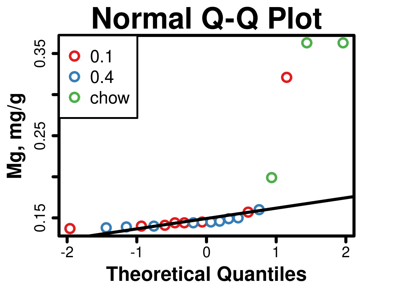
Cardiac magnesium levels from Smith BW J Food Res 2013 (doi: 10.5539/jfr.v2n1p168).

Import dataset

In RStudio, tools->import dataset can also be used.
Dataset is attached so variables can be named without reference to the original dataset.

cardiacMg <- read.table('data/kruskal_wallis_jfr2013_mg_cardiac.csv',
                        header = TRUE,
                        sep = ',')
attach(cardiacMg)

Perform Kruskal-Wallis test

# Convert independent variable to a factor for use later by PMCMRplus
cardiacMg$diet = as.factor(cardiacMg$diet)
# Perform Kruskal-Wallis test
kruskal.test(mg ~ diet, data = cardiacMg)

## 
##  Kruskal-Wallis rank sum test
## 
## data:  mg by diet
## Kruskal-Wallis chi-squared = 6.7757, df = 2, p-value = 0.03378

Multiple comparisons

Pairwise Wilcoxon testing with experiment-wide error correction
Nemenyi test (pairwise test for multiple comparisons of mean rank sums). Not corrected for multiple comparisons.
Dunnett non-parametric multiple comparisons

# Pairwise Wilcoxon
pairwise.wilcox.test(cardiacMg$mg, cardiacMg$diet, p.adjust.method = 'holm')

## Warning in wilcox.test.default(xi, xj, paired = paired, ...): cannot compute
## exact p-value with ties

## Warning in wilcox.test.default(xi, xj, paired = paired, ...): cannot compute
## exact p-value with ties

## Warning in wilcox.test.default(xi, xj, paired = paired, ...): cannot compute
## exact p-value with ties

## 
##  Pairwise comparisons using Wilcoxon rank sum test with continuity correction 
## 
## data:  cardiacMg$mg and cardiacMg$diet 
## 
##      0.1   0.4  
## 0.4  0.885 -    
## chow 0.063 0.048
## 
## P value adjustment method: holm

# Nemenyi
library(PMCMRplus)
kwAllPairsNemenyiTest(cardiacMg$mg, cardiacMg$diet, method = 'Tukey')

## Warning in kwAllPairsNemenyiTest.default(cardiacMg$mg, cardiacMg$diet, method =
## "Tukey"): Ties are present, p-values are not corrected.

## 
##  Pairwise comparisons using Tukey-Kramer-Nemenyi all-pairs test with Tukey-Dist approximation

## data: cardiacMg$mg and cardiacMg$diet

##      0.1   0.4  
## 0.4  0.992 -    
## chow 0.039 0.044

## 
## P value adjustment method: single-step

## alternative hypothesis: two.sided

# Dunnett
library(nparcomp)
nparcomp(mg ~ diet,
         data = cardiacMg,
         type = 'Dunnett',
         control = 'chow')

## 
##  #------Nonparametric Multiple Comparisons for relative contrast effects-----# 
##  
##  - Alternative Hypothesis:  True relative contrast effect p is not equal to 1/2 
##  - Type of Contrast : Dunnett 
##  - Confidence level: 95 % 
##  - Method = Logit - Transformation 
##  - Estimation Method: Pairwise rankings 
##  
##  #---------------------------Interpretation----------------------------------# 
##  p(a,b) > 1/2 : b tends to be larger than a 
##  #---------------------------------------------------------------------------# 
##

## $Data.Info
##   Sample Size
## 1    0.1    8
## 2    0.4    9
## 3   chow    3
## 
## $Contrast
##            0.1 0.4 chow
## 0.1 - chow   1   0   -1
## 0.4 - chow   0   1   -1
## 
## $Analysis
##        Comparison Estimator Lower Upper Statistic    p.Value
## 1 p( chow , 0.1 )     0.042 0.002 0.541 -2.124749 0.06608568
## 2 p( chow , 0.4 )     0.001 0.000 0.005 -9.757859 0.00000000
## 
## $Overall
##   Quantile p.Value
## 1 2.236422       0
## 
## $input
## $input$formula
## mg ~ diet
## 
## $input$data
##    diet    mg
## 1  chow 0.199
## 2  chow 0.363
## 3  chow 0.363
## 4   0.1 0.321
## 5   0.1 0.141
## 6   0.1 0.144
## 7   0.1 0.145
## 8   0.1 0.140
## 9   0.1 0.157
## 10  0.1 0.137
## 11  0.1 0.144
## 12  0.4 0.140
## 13  0.4 0.160
## 14  0.4 0.138
## 15  0.4 0.145
## 16  0.4 0.150
## 17  0.4 0.146
## 18  0.4 0.144
## 19  0.4 0.149
## 20  0.4 0.139
## 
## $input$type
## [1] "Dunnett"
## 
## $input$conf.level
## [1] 0.95
## 
## $input$alternative
## [1] "two.sided" "less"      "greater"  
## 
## $input$asy.method
## [1] "logit"  "probit" "normal" "mult.t"
## 
## $input$plot.simci
## [1] FALSE
## 
## $input$control
## [1] "chow"
## 
## $input$info
## [1] TRUE
## 
## $input$rounds
## [1] 3
## 
## $input$contrast.matrix
## NULL
## 
## $input$correlation
## [1] FALSE
## 
## $input$weight.matrix
## [1] FALSE
## 
## 
## $text.Output
## [1] "True relative contrast effect p is not equal to 1/2"
## 
## $connames
## [1] "p( chow , 0.1 )" "p( chow , 0.4 )"
## 
## $AsyMethod
## [1] "Logit - Transformation"
## 
## attr(,"class")
## [1] "nparcomp"

Test assumptions

Normality

The RColorBrewer package is loaded for additional colors, and a palette is added to R. Use brackets after vector name for specific colors when creating plots (for example: col=set1[4:14]).
Legend can also be manually positioned with xy coordinates (numbers from 0,0 at bottom left of plot to 1,1 at top right)
As demonstrated by the tests below, these data fail the assumption of normality, and are not amenable to transformation, hence the use of non-parametric testing.

# Shapiro-Wilk W test
shapiro.test(cardiacMg$mg)

## 
##  Shapiro-Wilk normality test
## 
## data:  cardiacMg$mg
## W = 0.55747, p-value = 1.101e-06

# Normal Quantile-Quantile Plot
# Set graphical parameters
par(
  cex = 1,
  cex.main = 3,
  cex.lab = 2,
  font.lab = 2,
  cex.axis = 1.5,
  lwd = 5,
  lend = 0,
  ljoin = 0,
  tcl = -0.5,
  pch = 1,
  mar = c(5, 5, 3, 5)
)

# Load RColorBrewer and set palette
library(RColorBrewer)
set1 <- brewer.pal(8, 'Set1')

# Create vector for categories
categories <- factor(cardiacMg$diet)

# Create plot
qqnorm(
  mg,
  ylab = 'Mg, mg/g',
  axes = FALSE,
  col = set1[categories],
  lwd = 4,
  cex = 2
)
# Add normal line
qqline(cardiacMg$mg, lwd = 5)
# Add border to complete axes
box(which = 'plot', bty = 'o', lwd = 5)
axis(1, lwd = 5, tcl = -0.5)  # x axis
axis(2, lwd = 5, tcl = -0.5)  # y axis
# Add legend
legend(
  'topleft',
  legend = levels(categories),
  box.lwd = 3,
  pch = 1.5,
  cex = 1.75,
  pt.cex = 2,
  pt.lwd = 4,
  col = set1
)

Equality of variances

This is a brown-forsythe test that evaluates deviations from group medians, and thus is robust to violations of normality.
Fligner test included for comparison.

library(lawstat)
levene.test(cardiacMg$mg, cardiacMg$diet)

## 
##  Modified robust Brown-Forsythe Levene-type test based on the absolute
##  deviations from the median
## 
## data:  cardiacMg$mg
## Test Statistic = 1.1301, p-value = 0.3461

# Fligner test
fligner.test(cardiacMg$mg ~ cardiacMg$diet)

## 
##  Fligner-Killeen test of homogeneity of variances
## 
## data:  cardiacMg$mg by cardiacMg$diet
## Fligner-Killeen:med chi-squared = 0.11837, df = 2, p-value = 0.9425

Generate boxplot

Parameters (par): Graphical parameters need to be set again because of code chunk separation in RMarkdown. Normally they would only be set once per R session.
X axis: The default axes will usually detect categorical data and label axes accordingly, but categories will need to be specified for axes created separately. It is easiest to create a separate vector with the categories, and then reference it when creating the plot. Labels can also be specified with labels=c('group1', 'group2').
Y axis: Note that it does not always start at zero, but encompasses the data range with some padding.

# Set graphical parameters
par(
  cex = 1,
  cex.main = 3,
  cex.lab = 2,
  font.lab = 2,
  cex.axis = 1.5,
  lwd = 5,
  lend = 0,
  ljoin = 0,
  tcl = -0.5,
  pch = 1,
  mar = c(5, 5, 3, 5)
)

# Create boxplot
boxplot(
  cardiacMg$mg ~ cardiacMg$diet,
  main = 'Cardiac mg',
  xlab = 'diet',
  ylab = 'Mg, mg/g',
  axes = FALSE,
  lwd = 4,
  medlwd = 7,
  outlwd = 4,
  cex = 2,
  col = set1
)

# Add border to complete axes
box(which = 'plot', bty = 'l', lwd = 5)

# Create vector with means of each group
means <- aggregate(mg ~ diet, data = cardiacMg, mean)
# Add points for group means to boxplot
points(
  means$mg,
  cex = 2,
  pch = 23,
  bg = 0,
  lwd = 4
)

# X axis
axis(
  1,
  lwd = 5,
  tcl = -0.5,
  labels = levels(categories),
  at = c(1:3)
)

# Y axis
axis(2, lwd = 5, tcl = -0.5)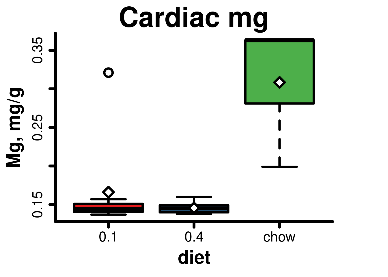

Plots

General examples

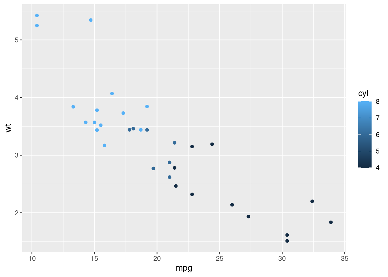
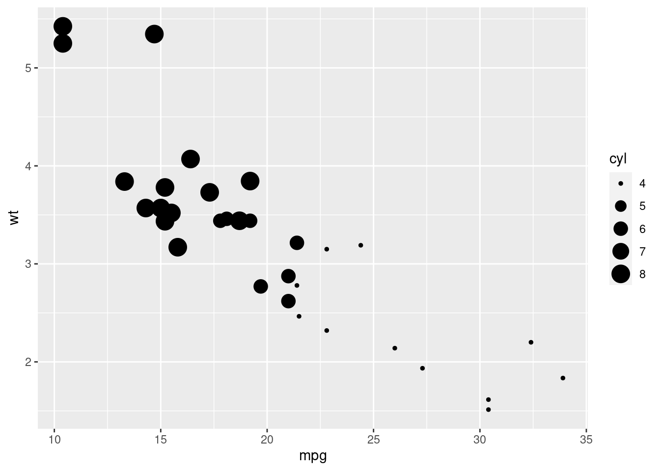
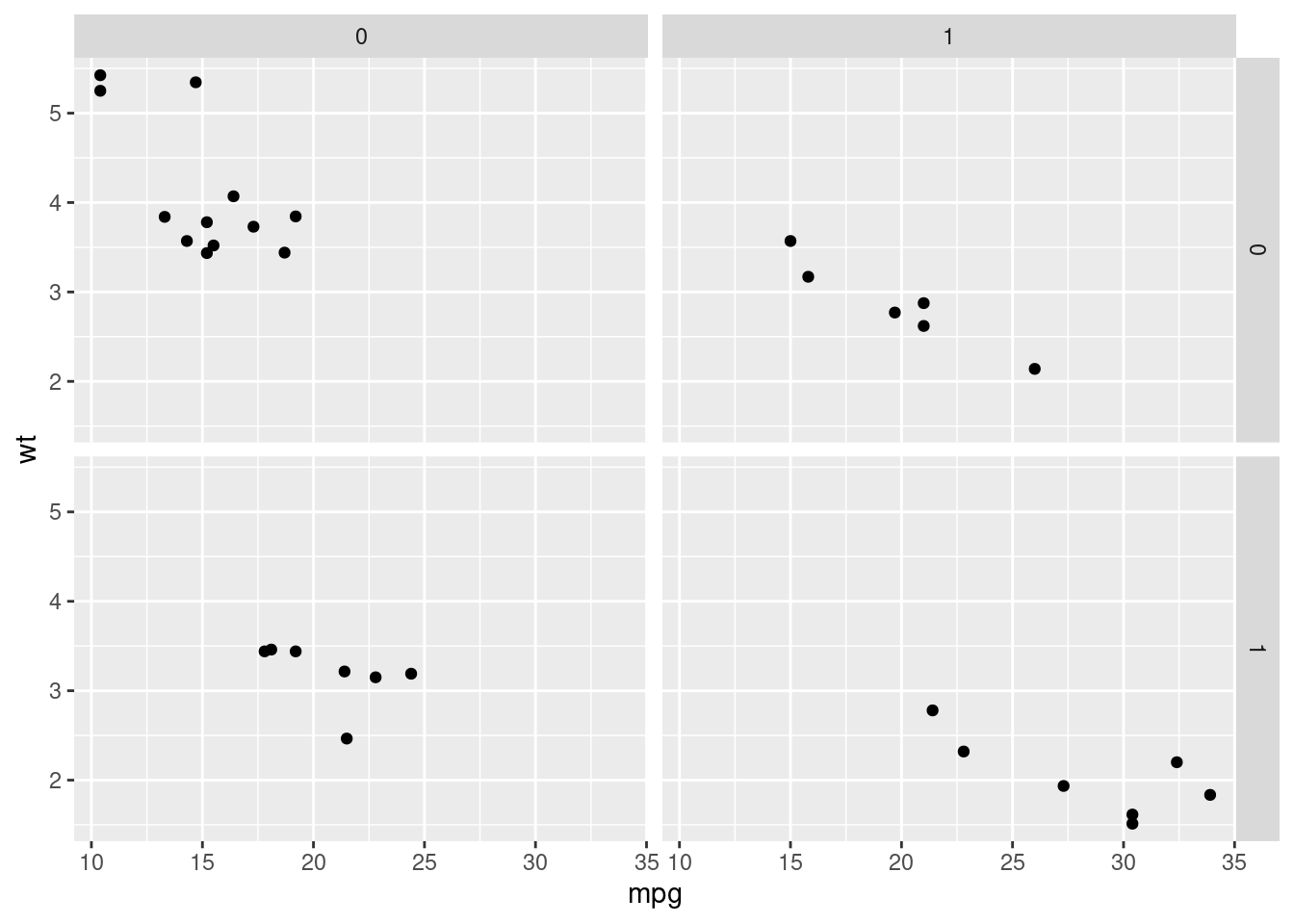
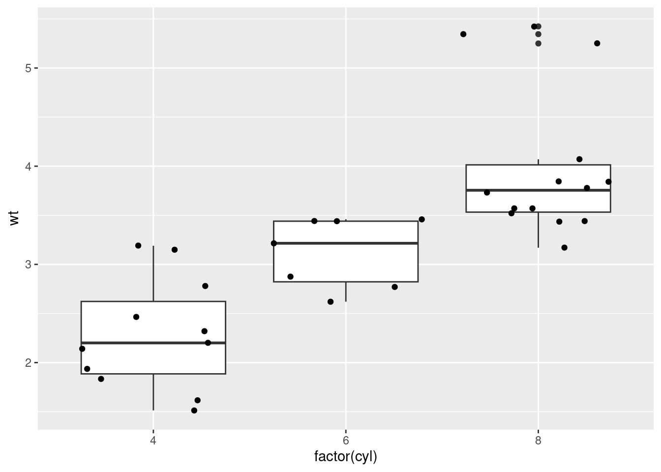
ggplot2 qplot example

Example from ggplot2 documentation p. 135

Intro

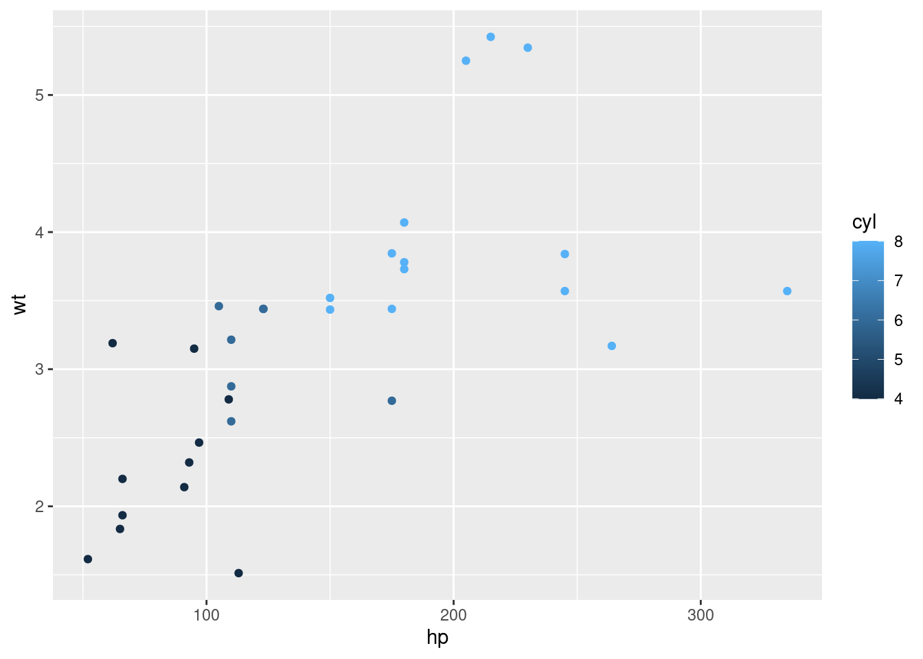
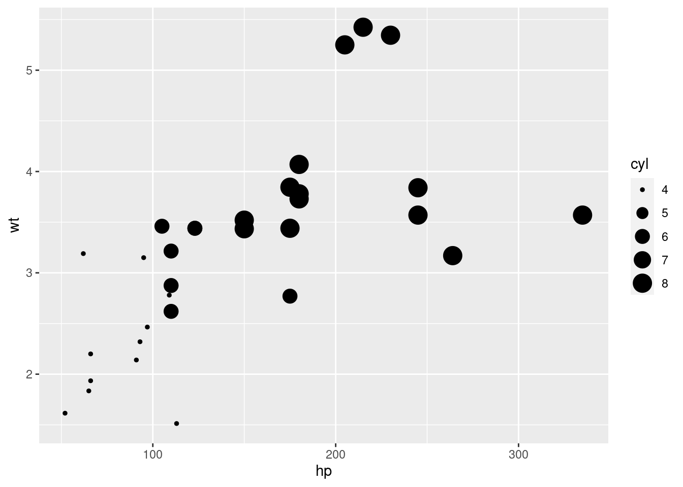
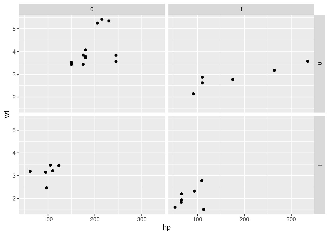
This file demonstrates some of the capabilities in the ggplot2 package. The mtcars dataset is included with R. The beginning of the dataset is shown with head(mtcars) to verify.

Import data

library(ggplot2)
head(mtcars)

##                    mpg cyl disp  hp drat    wt  qsec vs am gear carb
## Mazda RX4         21.0   6  160 110 3.90 2.620 16.46  0  1    4    4
## Mazda RX4 Wag     21.0   6  160 110 3.90 2.875 17.02  0  1    4    4
## Datsun 710        22.8   4  108  93 3.85 2.320 18.61  1  1    4    1
## Hornet 4 Drive    21.4   6  258 110 3.08 3.215 19.44  1  0    3    1
## Hornet Sportabout 18.7   8  360 175 3.15 3.440 17.02  0  0    3    2
## Valiant           18.1   6  225 105 2.76 3.460 20.22  1  0    3    1

Plot data

# from ggplot2 documentation p.135
# Use data from data.frame
qplot(mpg, wt, data = mtcars)

## Warning: `qplot()` was deprecated in ggplot2 3.4.0.
## This warning is displayed once every 8 hours.
## Call `lifecycle::last_lifecycle_warnings()` to see where this warning was
## generated.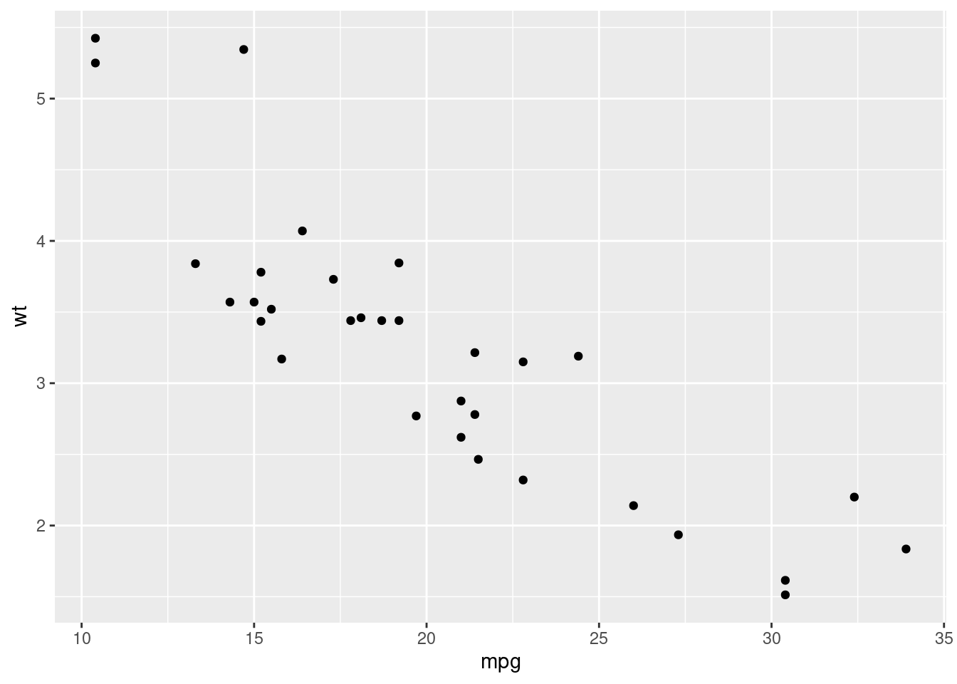

qplot(mpg, wt, data = mtcars, colour = cyl)

qplot(mpg, wt, data = mtcars, size = cyl)

qplot(mpg, wt, data = mtcars, facets = vs ~ am)

# It will use data from local environment
hp <- mtcars$hp
wt <- mtcars$wt
cyl <- mtcars$cyl
vs <- mtcars$vs
am <- mtcars$am
qplot(hp, wt)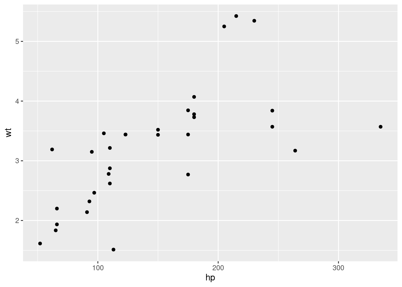

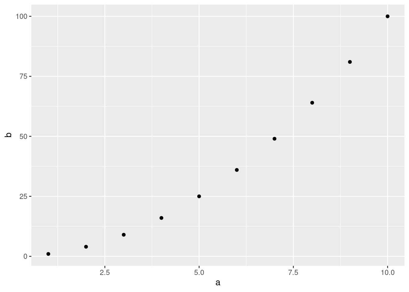
qplot(hp, wt, colour = cyl)

qplot(hp, wt, size = cyl)

qplot(hp, wt, facets = vs ~ am)

qplot(1:10, rnorm(10), colour = runif(10))

qplot(1:10, letters[1:10])

mod <- lm(mpg ~ wt, data = mtcars)
qplot(resid(mod), fitted(mod))

qplot(resid(mod), fitted(mod), facets = . ~ vs)

f <- function() {
  a <- 1:10
  b <- a ^ 2
  qplot(a, b)
}
f()

# qplot will attempt to guess what geom you want depending on the input
# both x and y supplied = scatterplot
qplot(mpg, wt, data = mtcars)

# just x supplied = histogram
qplot(mpg, data = mtcars)

## `stat_bin()` using `bins = 30`. Pick better value with `binwidth`.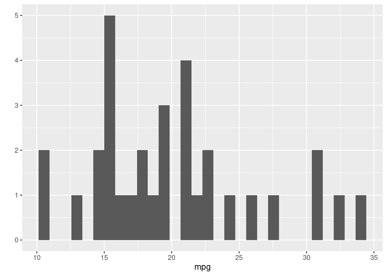

# just y supplied = scatterplot, with x = seq_along(y)
qplot(y = mpg, data = mtcars)

# Use different geoms
qplot(mpg, wt, data = mtcars, geom = 'path')

qplot(factor(cyl),
      wt,
      data = mtcars,
      geom = c('boxplot', 'jitter'))

qplot(mpg, data = mtcars, geom = 'dotplot')

## Bin width defaults to 1/30 of the range of the data. Pick better value with
## `binwidth`.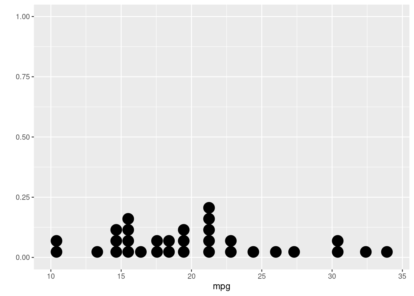

Creating rotated axis labels in R

7.27 How can I create rotated axis labels?

Intro

To rotate axis labels (using base graphics), you need to use text(), rather than mtext(), as the latter does not support par(‘srt’).

Example plot

# Increase bottom margin to make room for rotated labels
par(mar = c(7, 4, 4, 2) + 0.1)
# Create plot with no x axis and no x axis label
plot(1:8, xaxt = 'n',  xlab = '')
# Set up x axis with tick marks alone
axis(1, labels = FALSE)
# Create some text labels
labels <- paste('Label', 1:8, sep = ' ')
# Plot x axis labels at default tick marks
text(
  1:8,
  par('usr')[3] - 0.25,
  srt = 45,
  adj = 1,
  labels = labels,
  xpd = TRUE
)
# Plot x axis label at line 6 (of 7)
mtext(1, text = 'X Axis Label', line = 6)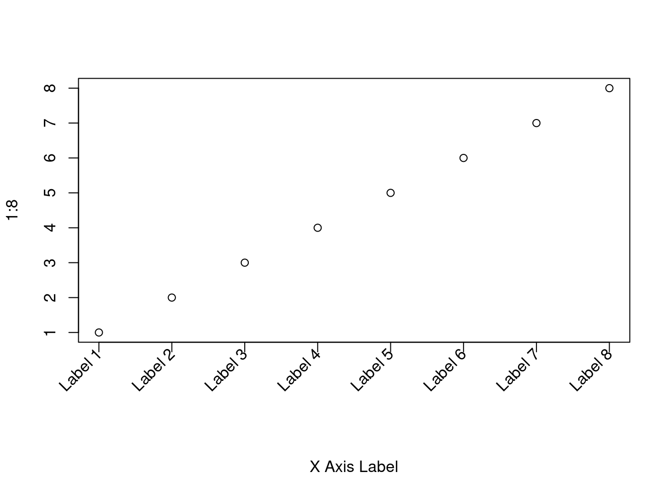

Comments

When plotting the x axis labels, we use srt = 45 for text rotation angle, adj = 1 to place the right end of text at the tick marks, and xpd = TRUE to allow for text outside the plot region. You can adjust the value of the 0.25 offset as required to move the axis labels up or down relative to the x axis. See ?par for more information.
Also see Figure 1 and associated code in Paul Murrell (2003), ‘Integrating grid Graphics Output with Base Graphics Output’, R News, 3/2, 7-12.

Volcano plots

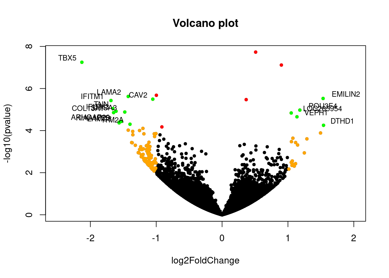
Getting Genetics Done example

Volcano plot example from Getting Genetics Done, with data from this GitHub Gist.

Import dataset from GitHub

res <- read.table('data/volcano_ggd_data.txt', header = TRUE)
head(res)

##      Gene log2FoldChange    pvalue      padj
## 1    DOK6         0.5100 1.861e-08 0.0003053
## 2    TBX5        -2.1290 5.655e-08 0.0004191
## 3 SLC32A1         0.9003 7.664e-08 0.0004191
## 4  IFITM1        -1.6870 3.735e-06 0.0068090
## 5   NUP93         0.3659 3.373e-06 0.0068090
## 6 EMILIN2         1.5340 2.976e-06 0.0068090

Make a basic volcano plot

The -log10(pvalue) is used so p values can be plotted as whole numbers. Note that I was not able to separate each section into different R markdown code chunks. I needed the generation of points to be continuous with generation of the original plot.

with(res,
     plot(
       log2FoldChange,
       -log10(pvalue),
       pch = 20,
       main = 'Volcano plot',
       xlim = c(-2.5, 2)
     ))
# Add colored points:
# red if padj<0.05
# orange if log2FC>1
# green if both
with(subset(res, padj < .05),
     points(
       log2FoldChange,
       -log10(pvalue),
       pch = 20,
       col = 'red'
     ))
with(subset(res, abs(log2FoldChange) > 1),
     points(
       log2FoldChange,
       -log10(pvalue),
       pch = 20,
       col = 'orange'
     ))
with(subset(res, padj < .05 & abs(log2FoldChange) > 1),
     points(
       log2FoldChange,
       -log10(pvalue),
       pch = 20,
       col = 'green'
     ))

# Label points with the textxy function from the calibrate package
library(calibrate)
with(subset(res, padj < .05 & abs(log2FoldChange) > 1),
     textxy(
       log2FoldChange,
       -log10(pvalue),
       labs = Gene,
       cex = .8
     ))

Nrf1 proteomics volcano plot

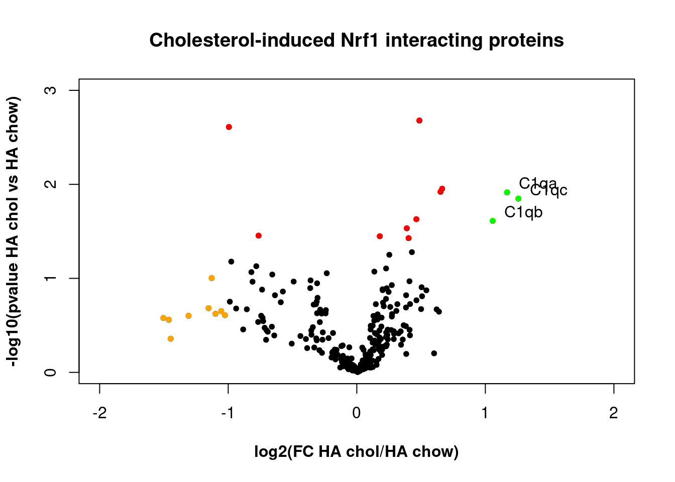
Experimental data example from Nrf1 proteomics project. The goal of this experiment was to identify a molecular complex associated with Nrf1, a protein molecule our research group was studying. Complement C1q proteins were identified as potentially interacting with Nrf1.

Import data

proteomics_data <-
  read.table(
    'https://raw.githubusercontent.com/br3ndonland/R-proteomics-Nrf1/master/data/R-proteomics-Nrf1.csv',
    header = TRUE,
    sep = ','
  )
attach(proteomics_data)
head(proteomics_data)

##       Gene log2_FC_HAchol_HAchow log2_FC_HAchow_lacZ     pvalue pvaluechow
## 1 Serpinb5            0.09538888          -1.3634997 0.74081917 0.39977101
## 2      Sfn            0.41354494          -1.0428302 0.40347276 0.20906780
## 3     Eno1            0.63929006          -0.6662456 0.22617602 0.32692726
## 4     C1qc            1.25725953           0.0891710 0.01419030 0.86011207
## 5     C1qa            1.16884182           0.0303050 0.01219113 0.95321354
## 6    Gstm1            0.19700734          -0.8650671 0.65225515 0.09657287
##   log2_FC_HAbort_HAchow pvaluebort
## 1             1.7303640 0.31471162
## 2             2.5999482 0.01377441
## 3             0.8034121 0.06946092
## 4             0.0946041 0.84034899
## 5             0.1015774 0.80231428
## 6             0.4450431 0.21202782

Generate plots

Each point is a protein.
- Red if p<0.05 for the comparison shown
- Orange if [log2 fold change]>1
- Green if both
log2 transformation is used to normalize positive and negative fold changes.
-log10(pvalue) is used so p values can be plotted as whole numbers.

HA cholesterol plot

This plot compares chow-fed mice with mice fed the Paigen diet to promote accumulation of cholesterol in the liver, and demonstrates the increased abundance of Complement C1qA, C1qB, and C1qC, in mice fed the Paigen diet.

# bold axis titles
par(font.lab = 2)

# create plot
with(
  proteomics_data,
  plot(
    log2_FC_HAchol_HAchow,
    -log10(pvalue),
    pch = 20,
    xlim = c(-2, 2),
    ylim = c(0, 3),
    yaxp = c(0, 3, 3),
    main = 'Cholesterol-induced Nrf1 interacting proteins',
    xlab = 'log2(FC HA chol/HA chow)',
    ylab = '-log10(pvalue HA chol vs HA chow)'
  )
)

# Add colored points:
# red if pvalue<0.05, orange if [log2FC]>1, green if both)
with(
  subset(proteomics_data, pvalue < .05),
  points(
    log2_FC_HAchol_HAchow,
    -log10(pvalue),
    pch = 20,
    col = 'red'
  )
)

with(
  subset(proteomics_data, abs(log2_FC_HAchol_HAchow) > 1),
  points(
    log2_FC_HAchol_HAchow,
    -log10(pvalue),
    pch = 20,
    col = 'orange'
  )
)

with(
  subset(proteomics_data, pvalue < .05 &
           abs(log2_FC_HAchol_HAchow) > 1),
  points(
    log2_FC_HAchol_HAchow,
    -log10(pvalue),
    pch = 20,
    col = 'green'
  )
)

# Label points with the textxy function from the calibrate package
library(calibrate)
with(
  subset(proteomics_data, pvalue < .05 &
           abs(log2_FC_HAchol_HAchow) > 1),
  textxy(
    log2_FC_HAchol_HAchow,
    -log10(pvalue),
    labs = Gene,
    cex = 1
  )
)

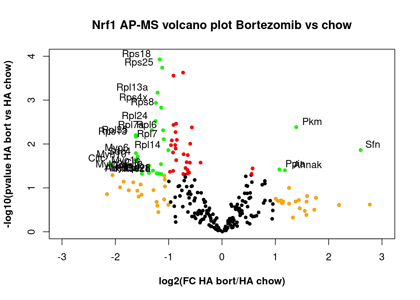
HA Bortezomib plot

Bortezomib treatment alters the proteome.

# bold axis titles
par(font.lab = 2)

# create plot
with(
  proteomics_data,
  plot(
    log2_FC_HAbort_HAchow,
    -log10(pvaluebort),
    pch = 20,
    xlim = c(-3, 3),
    ylim = c(0, 4),
    main = 'Nrf1 AP-MS volcano plot Bortezomib vs chow',
    xlab = 'log2(FC HA bort/HA chow)',
    ylab = '-log10(pvalue HA bort vs HA chow)'
  )
)
# Add colored points:
# red if pvalue<0.05, orange if log2FC>1, green if both)
with(
  subset(proteomics_data, pvaluebort < .05),
  points(
    log2_FC_HAbort_HAchow,
    -log10(pvaluebort),
    pch = 20,
    col = 'red'
  )
)

with(
  subset(proteomics_data, abs(log2_FC_HAbort_HAchow) > 1),
  points(
    log2_FC_HAbort_HAchow,
    -log10(pvaluebort),
    pch = 20,
    col = 'orange'
  )
)

with(
  subset(
    proteomics_data,
    pvaluebort < .05 & abs(log2_FC_HAbort_HAchow) > 1
  ),
  points(
    log2_FC_HAbort_HAchow,
    -log10(pvaluebort),
    pch = 20,
    col = 'green'
  )
)

# Label points with the textxy function from the calibrate package
library(calibrate)
with(
  subset(
    proteomics_data,
    pvaluebort < .05 & abs(log2_FC_HAbort_HAchow) > 1
  ),
  textxy(
    log2_FC_HAbort_HAchow,
    -log10(pvaluebort),
    labs = Gene,
    cex = 1
  )
)

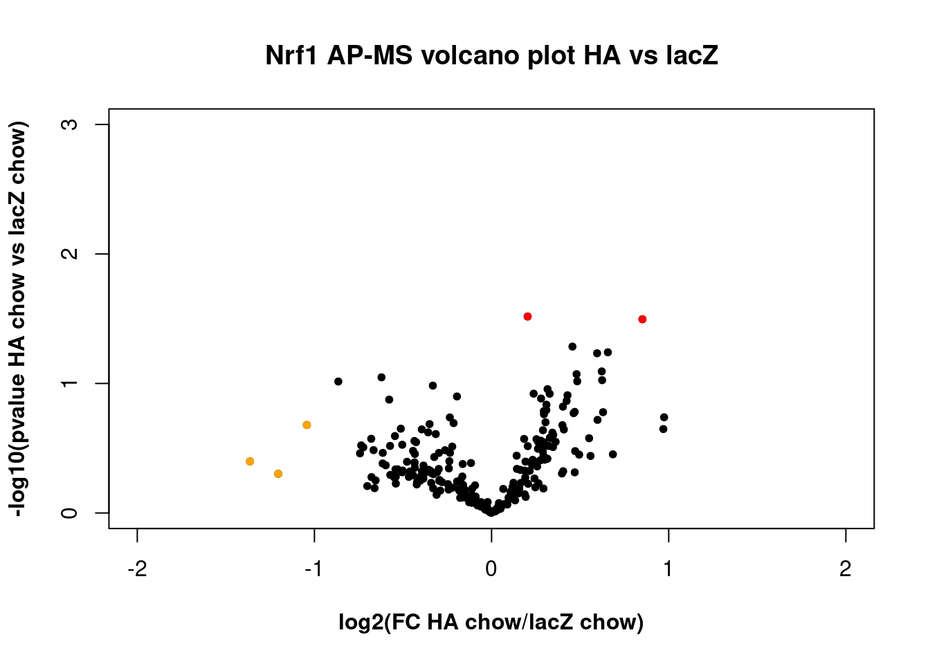
HA vs lacZ plot

The proteome was not significantly different with or without the HA tag, indicating issues with the HA immunoprecipitation. Note that the code for labeling points appears to be separated from the rest of the code for the plot, possibly because there were no points labeled.

# bold axis titles
par(font.lab = 2)

# create plot
with(
  proteomics_data,
  plot(
    log2_FC_HAchow_lacZ,-log10(pvaluechow),
    pch = 20,
    xlim = c(-2, 2),
    ylim = c(0, 3),
    yaxp = c(0, 3, 3),
    main = 'Nrf1 AP-MS volcano plot HA vs lacZ',
    xlab = 'log2(FC HA chow/lacZ chow)',
    ylab = '-log10(pvalue HA chow vs lacZ chow)'
  )
)

# Add colored points:
# red if pvalue<0.05, orange if [log2FC]>1, green if both)
with(
  subset(proteomics_data, pvaluechow < .05),
  points(
    log2_FC_HAchow_lacZ,-log10(pvaluechow),
    pch = 20,
    col = 'red'
  )
)

with(
  subset(proteomics_data, abs(log2_FC_HAchow_lacZ) > 1),
  points(
    log2_FC_HAchow_lacZ,-log10(pvaluechow),
    pch = 20,
    col = 'orange'
  )
)

with(
  subset(proteomics_data, pvaluechow < .05 &
           abs(log2_FC_HAchow_lacZ) > 1),
  points(
    log2_FC_HAchow_lacZ,-log10(pvaluechow),
    pch = 20,
    col = 'green'
  )
)

# Label points with the textxy function from the calibrate package
library(calibrate)
with(
  subset(proteomics_data, pvaluechow < .05 &
           abs(log2_FC_HAchow_lacZ) > 1),
  textxy(
    log2_FC_HAchow_lacZ,-log10(pvaluechow),
    labs = Gene,
    cex = 1
  )
)

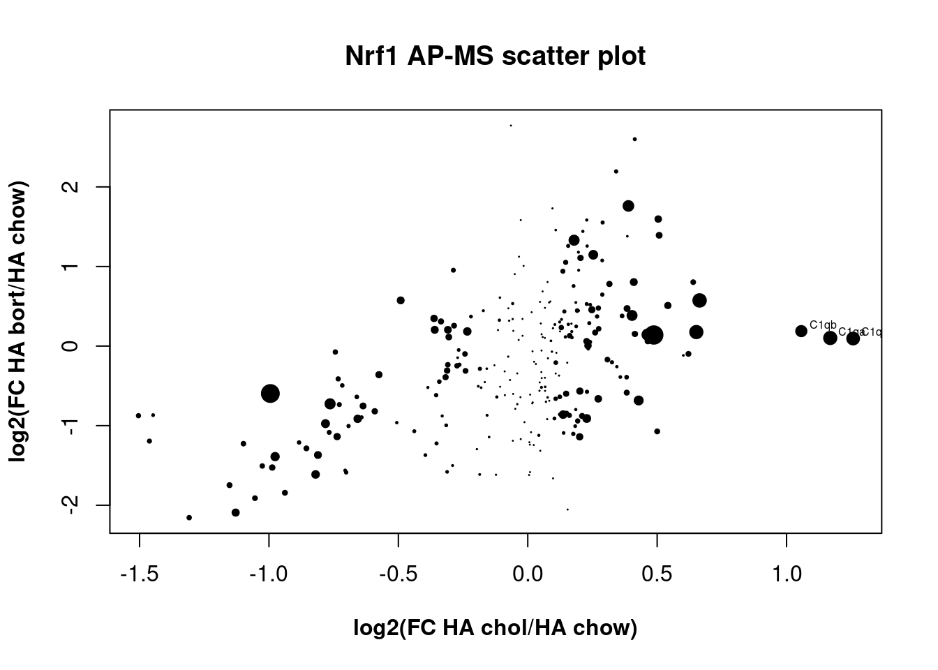
Scatter plot

The scatter plot is an interesting way to visualize two between-group comparisons, but the volcano plot is more useful for this dataset.

To set size of points according to p value:

dotsize <- -log10(pvalue)
head(dotsize)

then put cex=dotsize inside the plot() and points() functions.

# set size of points according to p value
dotsize <- -log10(pvalue)

# bold axis titles
par(font.lab = 2)

# create plot
with(
  proteomics_data,
  plot(
    log2_FC_HAchol_HAchow,
    log2_FC_HAbort_HAchow,
    pch = 20,
    main = 'Nrf1 AP-MS scatter plot',
    xlab = 'log2(FC HA chol/HA chow)',
    ylab = 'log2(FC HA bort/HA chow)',
    cex = dotsize
  )
)

# Label points with the textxy function from the calibrate package
library(calibrate)
with(
  subset(proteomics_data, pvalue < .05 &
           abs(log2_FC_HAchol_HAchow) > 1),
  textxy(log2_FC_HAchol_HAchow,
         log2_FC_HAbort_HAchow,
         labs = Gene)
)

R sample code

Brendon Smithbr3ndonlandSource code on GitHub

Data structures

Data frame

Example from Cookbook for R

Sample data frame

Sort data frame by column number

Sort data frame by column name

Example from Stack Overflow

Sample data frame

Sort data frame by column

Sort data frame by column index

Statistical models

T-test

Atheroma thickness

Import dataset

Perform t-test

Test assumptions

Normality

Equality of variances

Boxplot

Aorta Hsp70

Import dataset

Perform t-test

Test assumptions

Normality

Equality of variances

Boxplot

Linear regression

Simple linear regression aztcpm

Intro

Import dataset

Perform linear regression

Perform regression diagnostics and test assumptions

Generate plots

Log transform

Perform regression diagnostics and test assumptions

Generate plots

Simple linear regression jfs data

Import dataset

Perform linear regression

Perform regression diagnostics and test assumptions

Generate plots

Calculate Spearman correlation

Multiple linear regression and ANOVA example

Import dataset

Perform multiple linear regression in lm

Perform regression diagnostics and test assumptions

Generate plots

Perform ANOVA in aov for comparison

ANOVA

One-way ANOVA example

Import dataset

Perform ANOVA in aov

Perform multiple comparisons

Test assumptions

Normality

Equality of variances

Perform ANOVA in lm for comparison

Perform regression diagnostics and test assumptions

Two-way factorial ANOVA example

Load dataset

Perform factorial analysis of variance

Perform regression diagnostics and test assumptions

Generate plots

Two-way factorial ANOVA example

Import dataset

Perform factorial analysis of variance

Perform regression diagnostics and test assumptions

Generate plots

Log transform to correct non-normality, heteroscedasticity, and outlier

Perform regression diagnostics and test assumptions

Generate plots

ANOVA Compact Letter Display

Repeated measures ANOVA

Repeated measures ANOVA example

ANCOVA

One-way ANCOVA example

Load dataset

Perform analysis of covariance

Brendon Smith
br3ndonland
Source code on GitHub